The U.S. EPA introduced Method 200.7 to provide guidance on the use of ICP-OES in the determination of 30 different metals and trace elements in waters, wastewaters and solid wastes.1
Method 200.7 was introduced in 1994 and has seen routine implementation in environmental labs throughout the United States since.
Pollution and waste from industry continue to be produced in increasing quantities, necessitating the analysis of an increasing number of samples in line with Method 200.7.
Seeking to better meet this demand, PerkinElmer’s Avio® 560 Max fully simultaneous ICP-OES features a built-in High Throughput System (HTS) which enables rapid sample-to-sample times.
The HTS - a valve-and-loop system - utilizes a vacuum to rapidly fill and wash the sample loop, helping reduce the time needed for the sample to reach the nebulizer and minimize the washout time required after analysis.
This article builds on previous work,2 exploring the use of the Avio 560 Max ICP-OES in the analysis of wastewaters in line with Method 200.7.
Experimental
Samples and Sample Preparation
This methodology was developed and evaluated using four distinct wastewater certified reference materials:
- Wasterwaters C, D and H (High Purity Standards™, Charleston, South Carolina, USA)
- WasteWatR™, Trace Metals (ERA, Golden, Colorado, USA)
These standards were provided as concentrates, requiring them to be diluted as directed on their certificates. Samples were prepared in adherence to Method 200.7.
A total of 50 mL was acidified with 2 mL of 1:1 HNO3 and 1 mL of 1:1 HCl, before being placed in a hot block and heated to approximately 85 °C. Solutions were removed with around 20 mL final volume before being allowed to cool and then diluted to 50 mL using deionized water prior to analysis.
Table 1. Calibration Standards. Source: PerkinElmer, Inc.
| Element |
Standard 1 (mg/L) |
Standard 2 (mg/L) |
Ag, Al, As, B, Ba, Be, Cd, Co, Cr, Cu, Fe, Li, Mn,
Mo, Ni, P, Pb, Sb, Se, Si, Sn, Sr, Ti, Tl, V, Zn |
0.5 |
1 |
| Na, Mg, K, Ca |
10.5 |
21 |
Measurements were performed against external calibration curves, using standards prepared at a range of specific concentrations (Table 1) in 2% HNO3 (v/v). The internal standard (yttrium, Y) was prepared in 2% HNO3 (v/v) before being added to the sample stream via a port in the HTS valve.
All measurements were subjected to interelement corrections (IECs) and run at the concentrations defined in Method 200.7, except where these fell outside the linear range. In these instances, IEC solution concentrations were adjusted to fall within the linear range.
Instrumental Conditions
Analyses were performed using an Avio 560 Max ICP-OES, leveraging the High Throughput System (HTS)3 for sample introduction – this was also connected to an S23 Autosampler.
Table 2. Avio 560 Max ICP-OES with HTS Instrumental Parameters. Source: PerkinElmer, Inc.
| Paramenter/Component |
Value/Description |
| Sample Uptake Tubing |
Black/Black (0.76 mm id) PVC |
| Internal Standard Tubing |
Green/Orange (0.38 mm id), PVC |
| Drain Tubing |
Gray/Gray (1.30 mm id), Santoprene |
| Nebulizer |
MEINHARD® K1 |
| Spray Chamber |
Baffled Glass Cyclonic |
| Carrier |
2% HNO3 (v/v) |
| Carrier Flow Rate |
0.8 mL/min |
| Sample Loop Volume |
1 mL |
| Injector |
2.0 mm id Alumina |
| Nebulizer Gas Flow |
0.70 L/min |
| Auxiliary Gas Flow |
0.2 L/min |
| Plasma Gas Flow |
8 L/min |
| Torch Depth |
-3 |
| Integration |
Auto |
| Read Time Range |
0.5-5 sec |
| Loop Fill Time |
4 sec |
| Loop Rinse Time |
3 sec |
| Replicates |
2 |
Instrument parameters and conditions are displayed in Table 2, while analytes, analytical wavelengths and plasma view modes are listed in Table 3.
Table 3. Analytes, Wavelengths, and Plasma View Mode. Source: PerkinElmer, Inc.
| Element |
Wavelength (nm) |
Plasma View Mode |
| Ag |
328.068 |
Axial |
| Al |
308.215 |
Radial |
| As |
188.979 |
Axial |
| B |
249.677 |
Axial |
| Ba |
493.408 |
Radial |
| Be |
313.107 |
Radial |
| Ca |
315.887 |
Radial |
| Cd |
214.440 |
Axial |
| Ce |
413.764 |
Axial |
| Co |
228.616 |
Axial |
| Cr |
267.716 |
Axial |
| Cu |
324.752 |
Axial |
| Fe |
238.204 |
Radial |
| K |
766.490 |
Radial |
| Li |
670.784 |
Radial |
| Mg |
285.213 |
Radial |
| Mn |
257.610 |
Axial |
| Mo |
203.845 |
Axial |
| Na |
589.592 |
Radial |
| Ni |
231.604 |
Axial |
| P |
178.221 |
Axial |
| Pb |
220.353 |
Axial |
| Sb |
206.836 |
Axial |
| Se |
196.026 |
Axial |
| Si |
251.611 |
Radial |
| Sn |
189.927 |
Axial |
| Sr |
421.552 |
Radial |
| Ti |
334.940 |
Axial |
| Tl |
190.801 |
Axial |
| V |
292.402 |
Axial |
| Zn |
206.200 |
Axial |
| Y (Internal Standard) |
371.029 |
Axial and Radial |
The system employed a range of standard sample introduction components and conditions, including a total argon flow of 9 L/min.
Method 200.7 stipulates that four replicates should be utilized, but a common process employs only two or three replicates to improve sample throughput. To increase the relevance of this study to commercial labs, two replicates were utilized for every measurement.
The full range of analyses were performed using the auto-integration feature and a read-time range of between 0.5 and 5 seconds.
This approach ensured rapid analysis for high-level analytes while enabling low-level analytes to be measured accurately. Auto background correction was also used to streamline analysis.
Sample-to-sample time was approximately 60 seconds under these conditions. The sample-to-sample time varies depending on the analyte concentrations in the samples. To optimize performance, auto integration with varying read times was used.
Sample-to-sample time was, therefore, less than 60 seconds when working with higher concentrations, while sample-to-sample time was occasionally slightly longer than 60 seconds for samples with lower concentrations.
It is also possible to use three or four replicates to meet standard operating procedures with a minimal increase in sample-to-sample time.
Results and Discussion
To adhere to the guidelines established in Method 200.7, it is necessary to meet specific quality control (QC) criteria around sample handling/preparation and instrumental analysis.
Several criteria relate to instrumental analysis, and the study presented here aimed to determine the viability of the Avio 560 Max system in relation to these criteria;
- Linear dynamic range
- Method detection limits (MDLs)
- Instrument performance checks (IPCs)
- Spectral interference checks (SICs)
- Measurement accuracy
- Instrument stability
Facilitating Data Analysis with Smart Software
The Syngistix for ICP software (version 5.1 or higher) boasts an array of smart features designed to better facilitate data analysis and interpretation, for example, smart methods, smart workflow, smart monitoring and smart data. All these tools can be employed in the acquisition of data for Method 200.7.
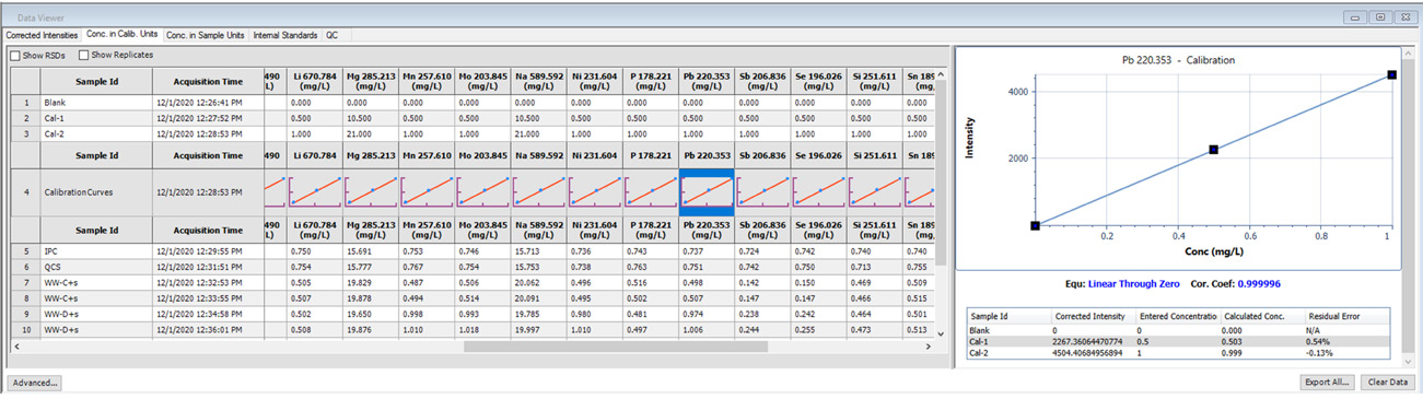
Figure 1. Calibration information displayed in Data Viewer. Image Credit: PerkinElmer, Inc.
Calibration curves are a key factor in the acquisition of robust data, and these must be reviewed to ensure good linearity – a task easily achieved using Data Viewer (Figure 1).
Data acquired in Data Viewer features thumbnails of the relevant calibration curves, allowing users a quick overview.
Clicking on a thumbnail provides expanded calibration curve details illustrating the equation, correlation coefficients, corrected intensities, entered and calculated concentrations for each standard, as well as the residual error for each individual standard.
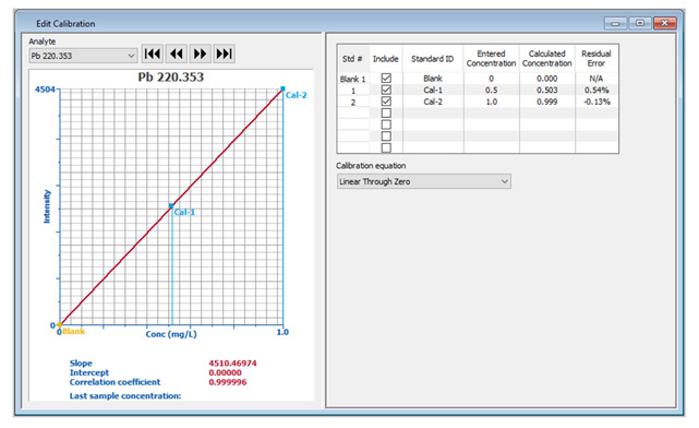
Figure 2. Detailed calibration information displayed in the Edit Calibration window. Image Credit: PerkinElmer, Inc.
If the calibration curve requires modification (for example, due to an out-of-range standard), the same comprehensive information can be seen in the Edit Calibration window (Figure 2), allowing easy editing of calibration information.
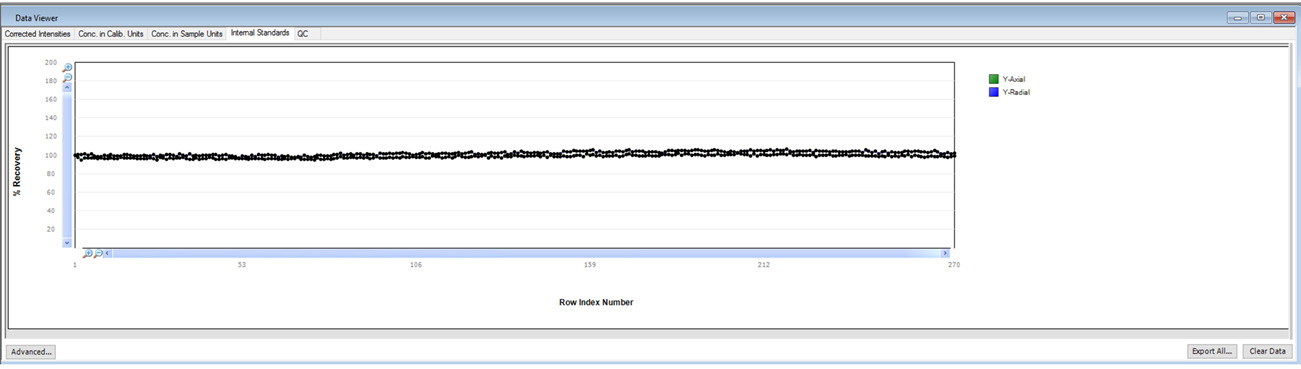
Figure 3. Internal standard plot in Data Viewer. Image Credit: PerkinElmer, Inc.
It is also important to monitor internal standard stability, particularly when running long-term stability testing. The normalized internal standard response (normalized to the calibration blank) is displayed in Data Viewer in real-time (Figure 3).
This useful feature allows the user to monitor the real-time performance of an active run effectively.
Initial QC: Initial Performance Check and Quality Control Sample
An initial performance check (IPC) should be analyzed immediately following the calibration to confirm the calibration curve’s quality. It is important to ensure that the IPC is a separate standard created from the same stock standard as the calibration standards.
A quality control sample (QCS) should also be made to an identical concentration as the IPC but from a second-source standard to validate the concentrations of stock solutions employed in the calibration standards.
Before the analysis can proceed, it is important that both the IPC and QCS recover within 5% of their true values.
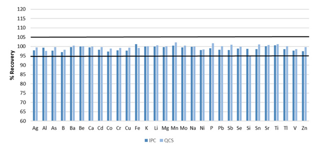
Figure 4. Recoveries for initial IPC and QCS. Image Credit: PerkinElmer, Inc.
All elements were found to be present at 0.75 ppm for the examples presented here, other than the minerals (Ca, K, Mg, Na), which were added at 21 ppm. The QCS and IPC were both found to recovered within the required 5% for all analytes (Figure 4).
Method Detection Limits
Method 200.7 stipulates that method detection limits (MDLs) should be determined by spiking a standard with analytes at two or three times the instrumental detection limits (IDLs) and measuring this a total of seven times.
Once the seven measurements have been acquired, the standard deviation should be multiplied by 3.14 to obtain MDLs at the 99% confidence level.
The IDLs must be determined before MDLs can be measured, with IDLs calculated by multiplying the standard deviation of ten blank measurements by three.
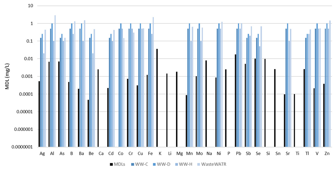
Figure 5. Method detection limits (black) along with certified concentrations in four reference materials (shades of blue). Not all analytes were certified in the reference materials. Image Credit: PerkinElmer, Inc.
Figure 5 displays MDLs plotted alongside certified analyte concentrations for the four reference materials analyzed. It should be noted that not every analyte was included in the reference materials.
The MDLs were found to be considerably lower than the certified values, illustrating the methodology’s capacity to easily measure low-level analytes in wastewaters.
Linear Dynamic Range
Method 200.7 regards the linear dynamic range as the highest concentration, which recovers within 10% of its true value when measured against the calibration curve employed in the analysis.
All linear dynamic range measurements performed in this study were conducted in multi-element solutions to increase their relevance to sample analyses, which are consistently multi-element solutions in practice.
Table 4. Linear Dynamic Range. Source: PerkinElmer, Inc.
| Elements |
Linear Range (mg/L) |
| Cd, Mn, Sr |
30 |
| Ba |
40 |
| Co, Cr, Ni, Sn, Ti, Tl |
50 |
| Be |
70 |
| Ag, Al, As, B, Cu, Fe, Li, Mg, Mo, P, Pb, Sb, Se, Si, V, Zn |
100* |
| Ca, K, Na |
500* |
*= highest concentration evaluated
The linear dynamic range is the highest concentration analyzed for most elements (Table 4), though the figures presented here represent the highest typical concentrations in wastewaters, rather than the limit of the Avio 560 Max ICP-OES itself.
It is possible to further extend the linear range of the Avio 560 Max by selecting less sensitive wavelengths, altering the torch position, changing the viewing height in the plasma to radial mode, changing the plasma viewing mode (for example, axial/radial), utilizing high-resolution mode and/or employing a less sensitive sample introduction system.
Accuracy
Having established the core characteristics of the methodology, it was necessary to ascertain its accuracy via the analysis of four reference materials with known, certified values (Table 5).
Table 5. Certified Values in Wastewater Reference Materials (all units in mg/L). Source: PerkinElmer, Inc.
| Element |
Wastewater C |
Wastewater D |
Wastewater H |
WasteWATR |
| Ag |
0.15 |
0.25 |
0.02 |
0.444 |
| Al |
0.5 |
1 |
0.1 |
2.91 |
| As |
0.15 |
0.25 |
0.1 |
0.151 |
| B |
0.5 |
1 |
0.25 |
1.33 |
| Ba |
0.5 |
1 |
0.1 |
1.5 |
| Be |
0.15 |
0.25 |
0.02 |
0.468 |
| Cd |
0.15 |
0.25 |
0.1 |
0.430 |
| Co |
0.5 |
1 |
0.5 |
0.147 |
| Cr |
0.5 |
1 |
0.5 |
0.302 |
| Cu |
0.5 |
1 |
0.5 |
0.526 |
| Fe |
0.5 |
1 |
0.25 |
2.25 |
| Mn |
0.5 |
1 |
0.1 |
0.636 |
| Mo |
0.5 |
1 |
0.1 |
0.578 |
| Ni |
0.5 |
1 |
0.5 |
1.21 |
| Pb |
0.5 |
1 |
0.5 |
1.05 |
| Sb |
0.15 |
0.25 |
0.2 |
0.693 |
| Se |
0.15 |
0.25 |
0.05 |
0.678 |
| Sr |
0.5 |
1 |
0.1 |
0.489 |
| Tl |
0.15 |
0.25 |
0.25 |
0.461 |
| V |
0.5 |
1 |
0.5 |
0.525 |
| Zn |
0.5 |
1 |
0.5 |
1.46 |
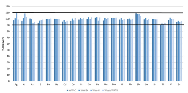
Figure 6. Certified analyte recoveries in four different wastewater reference materials. Image Credit: PerkinElmer, Inc.
Analyte recoveries for all certified elements were found to be within 10% of their certified values (Figure 6), therefore, confirming the accuracy of the methodology.
Table 6. Spiked Concentrations of Non-Certified Elements in Wastewater CRMs. Source: PerkinElmer, Inc.
| Analyte |
Concentration (mg/L) |
| Li, P, Si, Sn, Ti |
0.75 |
| Ca, K, Mg, Na |
20 |
Not every element discussed in Method 200.7 was certified in the reference materials; however, requiring these to be spiked into the reference materials at specific concentrations (Table 6) prior to digestion.
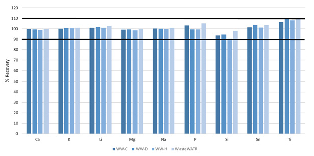
Figure 7. Recoveries of non-certified elements spiked into four wastewater CRMs. Image Credit: PerkinElmer, Inc.
These elements’ recoveries were also found to be within 10% of their true values (Figure 7), further illustrating the methodology’s accuracy.
Stability
With its accuracy confidently established, the methodology’s stability was determined via the measurement of wastewater samples and the monitoring of IPC standard recoveries, which were run every 10 samples.
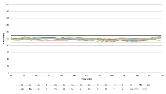
Figure 8. IPC recoveries during a 4-hour run of wastewaters, with a sample-to-sample time of ≈ 60 seconds. Image Credit: PerkinElmer, Inc.
All IPCs were found to recover within 10% of their certified values over the course of the 4-hour run (Figure 8), with a sample-to-sample time averaging 1 minute. These results highlight the exceptional stability of the system, even when working with a rapid sample-to-sample time of approximately 60 seconds.
This excellent stability was also afforded by a range of instrumental design considerations, including the vertical torch and Flat Plate™ plasma technology.
Measurements also took advantage of the dual view capability, allowing users to continuously switch between radial and axial plasma viewing modes for each sample.
Conclusion
The study presented here was successful in showcasing the Avio 560 Max ICP-OES’ capacity to perform rapid analysis – with an average sample-to-sample time of 60 seconds – of wastewater in adherence with the guidelines outlined in U.S. EPA Method 200.7.
The Avio 560 Max ICP-OES boasts exceptional accuracy, reliability, robustness and stability. These characteristics were demonstrated via the analysis of reference materials and QC checks.
The instrument’s built-in HTS offers a robust solution for wastewater analysis while using a total argon flow of 9 L/min to ensure a more rapid return on investment for all laboratories.
The HTS also substantially lowers sample uptake and washout times versus traditional sample introduction, increasing sample throughput even further.
References
- Method 200.7, Revision 4.4: Determination of Metals and Trace Elements in Water and Wastes by Inductively Coupled Plasma- Atomic Emission Spectrometry”, United States Environmental Protection Agency, 1994.
- “Analysis of Wastewaters Following U.S. EPA 200.7 using the Avio 550 Max ICP-OES”, Application Note, PerkinElmer Inc., 2020.
- “High Throughput System for ICP-MS/OES”, Product Note, PerkinElmer Inc., 2020.
Consumables Used
Table 7. Source: PerkinElmer, Inc.
| Component |
Part Number |
| Sample Uptake Tubing, Black/Black, (0.76 mm id), PVC, flared |
N8152407 |
| Internal Standard Tubing, Orange/Green (0.38 mm id), PVC, flared |
N8152403 |
| Drain Tubing, Gray/Gray (1.30 mm id), Santoprene |
N8152415 |
| Instrument Calibration Standard 1: 5000 mg/L Ca, K, Mg, Na |
N9300218 (125 mL) |
| Instrument Calibration Standard 2: 100 mg/L Ag, Al, As, Ba, Be, Ca, Cd, Co, Cr, Cu, Fe, K, Mg, Mn, Mo, Na, Ni, Pb, Sb, Se, Sn, Sr, Ti, Tl, V, Zn |
N9301721 (125 mL) |
| Boron Standard, 1000 mg/L |
N9300016 (125 mL)
N9303760 (500 mL) |
| Lithium Standard, 1000 mg/L |
N9303781 (125 mL)
N9300129 (500 mL) |
| Phosphorus Standard, 1000 mg/L |
N9303788 (125 mL)
N9300139 (500 mL) |
| Silicon Standard, 1000 mg/L |
N9303799 (125 mL)
N9300150 (500 mL) |
| Yttrium Standard, 1000 mg/L |
N9303810 (125 mL)
N9300167 (500 mL) |
| DigiTUBES, 50 mL |
N9308008 (Racklock with caps)
N9308340 (Racklock without caps)
N9308037 (non-Racklock with caps) |
| Autosampler Tubes |
B0193233 (15 mL)
B0193234 (50 mL) |
Acknowledgments
Produced from materials originally authored by Ken Neubauer from PerkinElmer, Inc.

This information has been sourced, reviewed and adapted from materials provided by PerkinElmer, Inc.
For more information on this source, please visit PerkinElmer, Inc.