The Red Sea basin is a biodiversity hotspot and small variations in climate change make a huge impact. The phytoplanktons of the area play a major role in the marine ecosystem and hence the phytoplankton phenology needs to be sustained. Kheireddine, M. et al. recently published a study detailing the use of a clustering technique to better comprehend the factors regulating the phytoplankton phenology.
Image Credit: Boris Stroujko/Shutterstock.com
The Red Sea, a marine biodiversity hotspot is enclosed by mangroves and coral reefs favoring the formation of specific ecological niches. The phytoplanktons present in this basin play a major role in the pelagic marine ecosystem's functioning. The phytoplankton cells also impact the production and vertical export of organic carbon—a major component of the carbon cycle influencing the atmospheric concentration of CO2.
Recent research works have revealed that the Red Sea is a quickly warming region of the global ocean, which likely affects the dynamic of the phytoplankton, particularly its phenology. This would in turn impact marine food webs and the efficacy of the biological carbon pump. The changes in phytoplankton phenology might induce a mismatch between primary producers, grazers, and apex predators which affects the export of organic carbon aggregates.
As the Red Sea is a small, semi-enclosed basin and these alterations affect the whole ecosystem, there is an enormous interest in understanding phytoplankton dynamics, and the Red Sea is considered to be the natural laboratory as this oceanic basin has conditions occurring in various tropical areas of the global ocean.
Some studies attempted to examine the phytoplankton phenology in the Red Sea and one study pinpointed the use of ocean color remote sensing as a robust tool to analyze the water column dynamics and the phytoplankton phenology. The study utilized ocean color remote sensing findings of chlorophyll-a concentration (CHL) to analyze Red Sea phytoplankton phenology.
The current research reinvestigates the ocean color remote sensing dataset of CHL to offer information on phytoplankton phenology in various areas of the basin using a prior method which was proved efficient. The study pinpoints bio-regions depending on observed annual cycles of phytoplankton biomass and puts forth mechanisms enhancing the phytoplankton dynamic and its inter-annual variability.
Methodology
Ocean color measurements of CHL were obtained from the Ocean Colour Climate Change Initiative (OC-CCI). Satellite images from 1998–2018 were collected. The researchers started with the regionalization of the Red Sea basin utilizing eight-day climatological satellite composite images of CHL. Pixels with the same CHL annual cycle were grouped into clusters that are defined as distinct bio-regions.
The temporal gaps were filled by a linear interpolation method. A cluster center was outlined as the mean of all CHL annual cycles and some phytoplankton phenology metrics were obtained from the four cluster centers—bloom initiation, termination and duration, and its maximum intensity utilizing the threshold criterion.
Later, annual datasets of normalized CHL cycles were clusterized and each yearly annual cycle was normalized by its maximum value. The yearly clustering of the Red Sea was carried out only in the north of the Red Sea. The R scripts utilized to carry out these clustering analyses are made publicly available on GitHub.
The Mixed Layer Depth (MLD) information from the Mercator model and the monthly values of the multivariable El Niño Southern Oscillation (ENSO) Index (MEI) were downloaded.
Results and Discussion
The climatological clustering method pinpointed four diverse bio-regions in the Red Sea (see Figure and Table 1). The presence of these bio-regions indicates high variability in the annual cycle of phytoplankton biomass. The spatial distribution also indicates that the dynamics might be due to the basin circulation dynamic and/or the accessibility of nutrients.
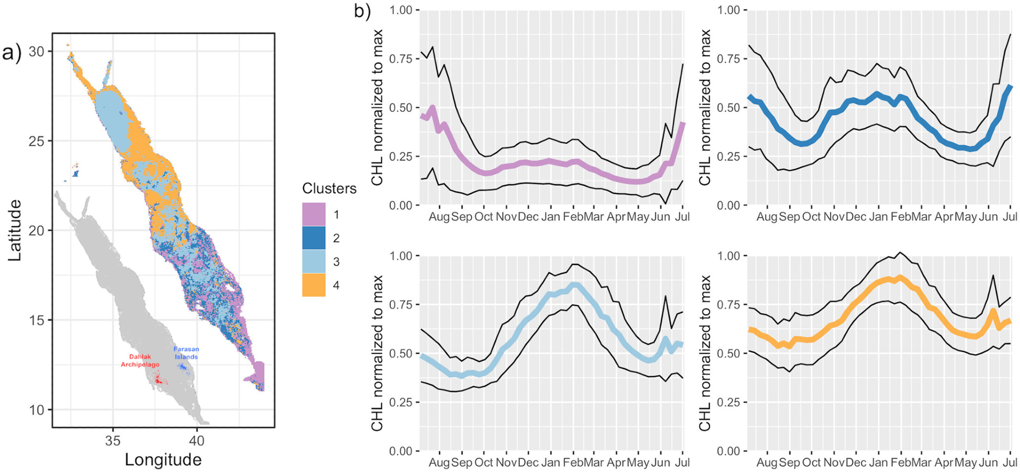
Figure 1. Regionalization of the phytoplankton phenology in the Red Sea. (a) Spatial distribution of the four bio-regions obtained with a fuzzy c-means clustering method applied to a dataset of climatological annual cycles of normalized CHL. (b) Annual cycle of normalized CHL of each bio-region. Thick lines depict averages and thin lines indicate the 1σ intervals. Image Credit: Kheireddine, et al., 2021
Table 1. Main characteristics of each Bio-region presented in Figure 1. Source: Kheireddine, et al., 2021
| Characteristics |
Bio-region 1 |
Bio-region 2 |
Bio-region 3 |
Bio-region 4 |
| Spatial distribution |
Southern Red
Sea |
Southern Red
Sea |
Northern Red
Sea |
Northern Red
Sea |
Around the Farasan islands and the Dahlak Archipelago |
The extreme northern Red Sea and the Gulf of Aqaba |
The north central Red Sea, The Northwestern coast and the Gulf of Suez |
| Phytoplankton bloom |
Summer bloom (July–August) |
Summer & Fall-Winter blooms (July) (November–February) |
Winter bloom (November–February) |
No winter bloom? (November–February) |
(Racault et al., 2015) |
(Racault et al., 2015) |
(Kheireddine et al., 2020) |
(Zarokanellos and Jones, 2021) |
| Seasonality (mg m-3) |
Median (Min. to Max.) |
Median (Min. to Max.) |
Median (Min. to Max.) |
Median (Min. to Max.) |
3.5 (0.36 to
13.07) |
0.96 (0.2 to
4.05) |
0.19 (0.12 to
0.50) |
0.13 (0.06 to
0.25) |
| Annual CHL (mg m-3) |
0.65 (0.02 to
2.23) |
0.57 (0.005 to
2.1) |
0.19 (0.004 to
0.51) |
0.18 (0.06 to
0.44) |
| Annual MLD (m) |
11 (8 to 16) |
15 (7 to 22) |
34 (11 to 71) |
25 (11 to 50) |
| Source of nutrients |
Southwest monsoon (Intrusion of sub-surface nutrient-rich waters from the Gulf of Aden) (Churchill et al., 2014) |
Southwest & Northeast Monsoons (Intrusion of sub-surface & surface nutrient-rich waters from the Gulf of Aden) (Churchill et al., 2014) |
Mixing events supplying nutrients in the surface layer (Kheireddine et al., 2020 and references therein) |
No nutrients (Dispersion of the subsurface chlorophyll maximum) (Zarokanellos and Jones, 2021) |
| Dominant Phytoplankton functional types |
Winter/Spring/Summer/Fall |
Micro-/Nano-/Micro/Micro-phytoplankton
(Brewin et al., 2015) |
Micro-/Nano-/Pico/Pico-phytoplankton
(Brewin et al., 2015) |
Figure 2 illustrates the phytoplankton phenology between these bio-regions.
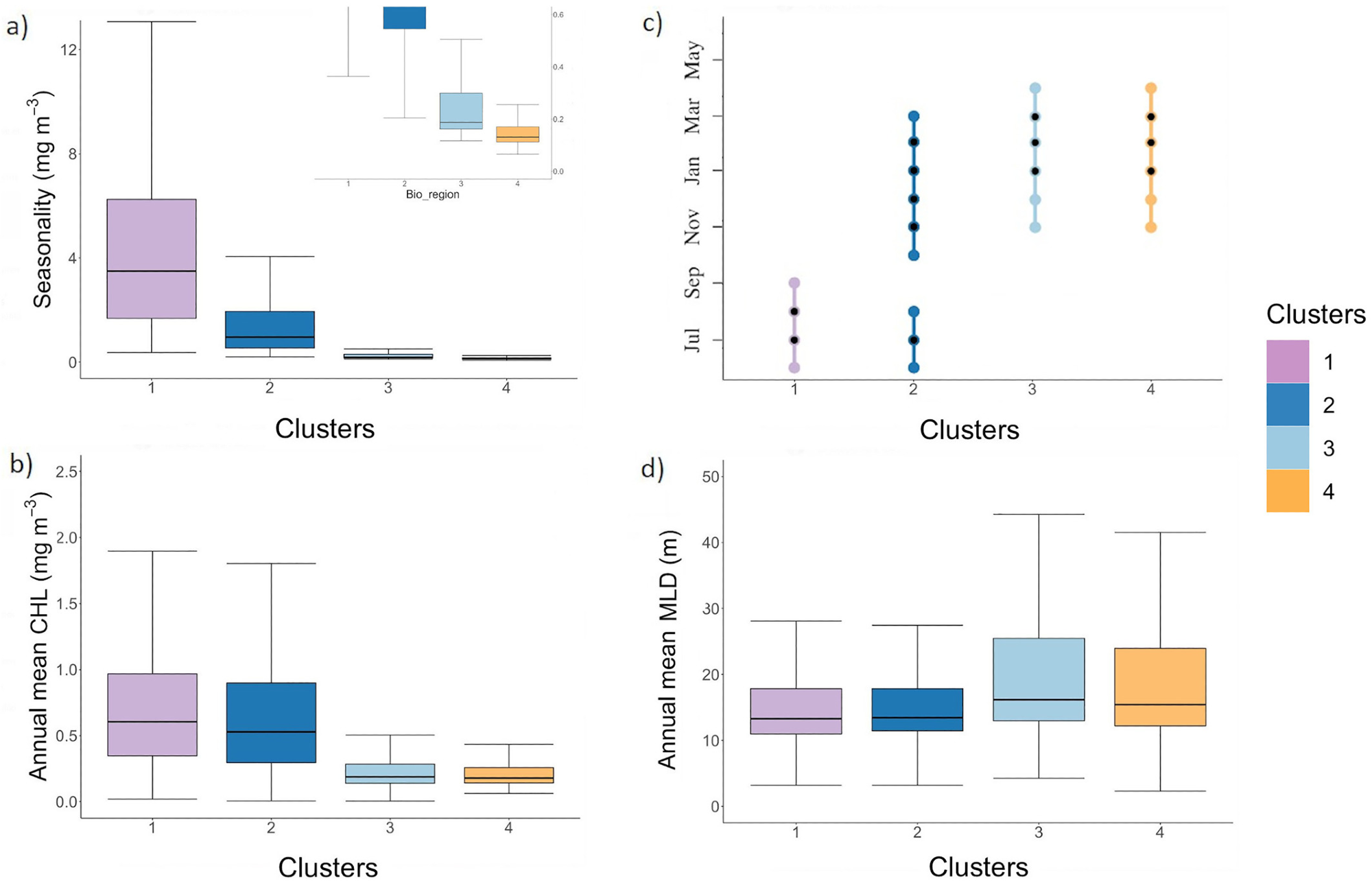
Figure 2. The chlorophyll-a seasonality (i.e., amplitude) (mg m−3) associated to a zoom on Bio-regions 3 and 4 (a), the annual mean chlorophyll-a concentration (mg m−3), the timing of the bloom maximum where the black dots correspond to the most frequent month where we observed the highest bloom intensity (month; y-axis) (c) and annual mean MLD (d). Image Credit: Kheireddine, et al., 2021
It was observed that Bio-regions 3 and 4 were predominant in the northern half of the Red Sea basin. The annual cycle associated with Bio-region 3 and 4 varied owing to the differences in air-sea heat fluxes and the dynamics of the basin. The phytoplankton seasonal cycle seen in Bio-region 3 was related to vertical mixing taking place in winter (see Figures 2d and 3).
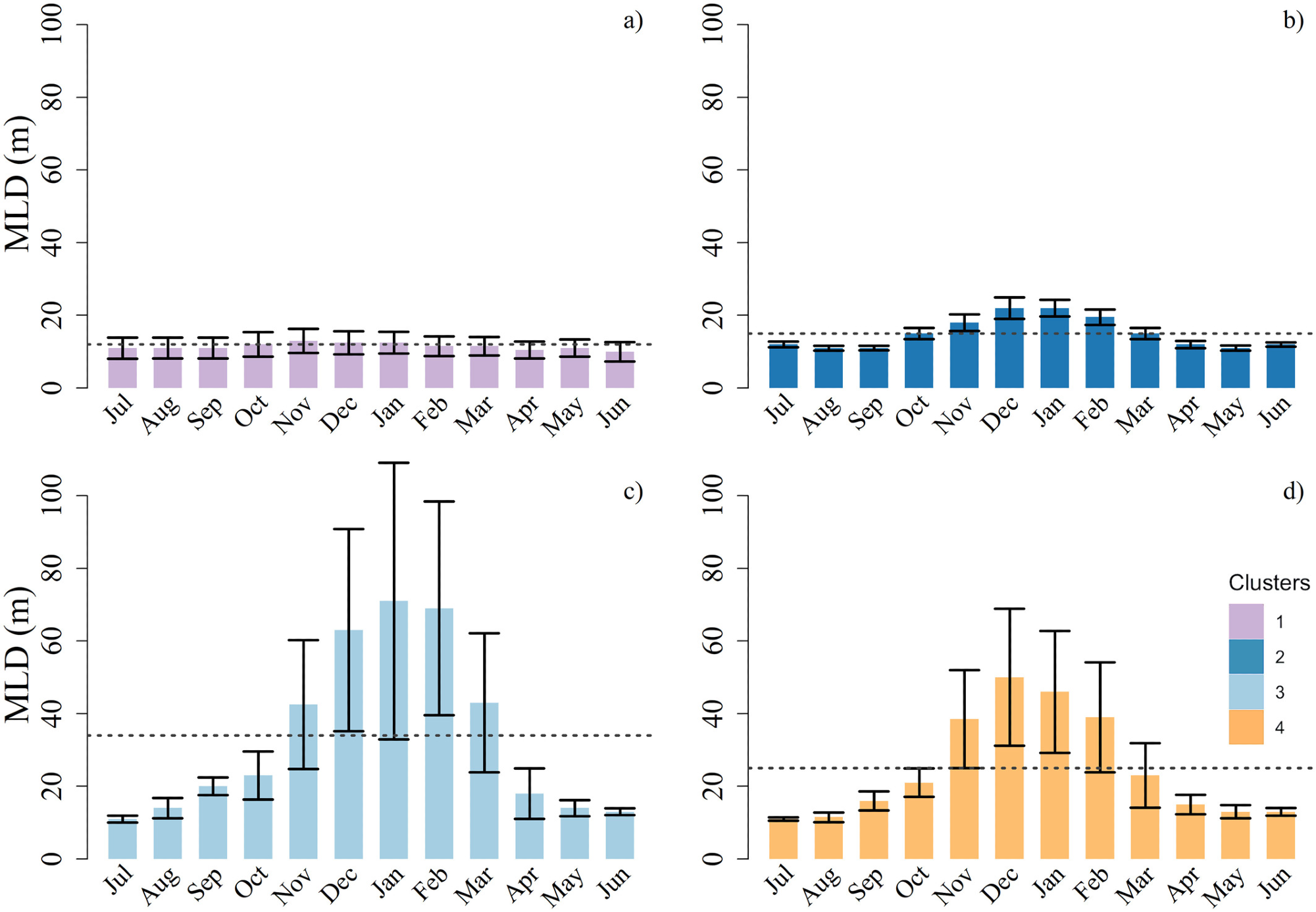
Figure 3. For each bio-region, average ± standard deviation of the annual cycles of the mixed layer depth (MLD). The dashed dark gray line represents the yearly average value of the MLD. Image Credit: Kheireddine, et al., 2021
The Bio-regions 3 and 4 also showed a recurrent summer peak in CHL in June, which might be due to the presence of anti-cyclonic mesoscale eddies. The spatial distribution of the bio-regions was greatly erratic with three bio-regions (Bio-regions 1, 2, and 3) in the southern half of the Red Sea.
Even though Bio-region 3 was found in the southern part of the basin, the core was seen in the northern part (see Figure 4) and its presence in the southern areas may be due to mesoscale features.
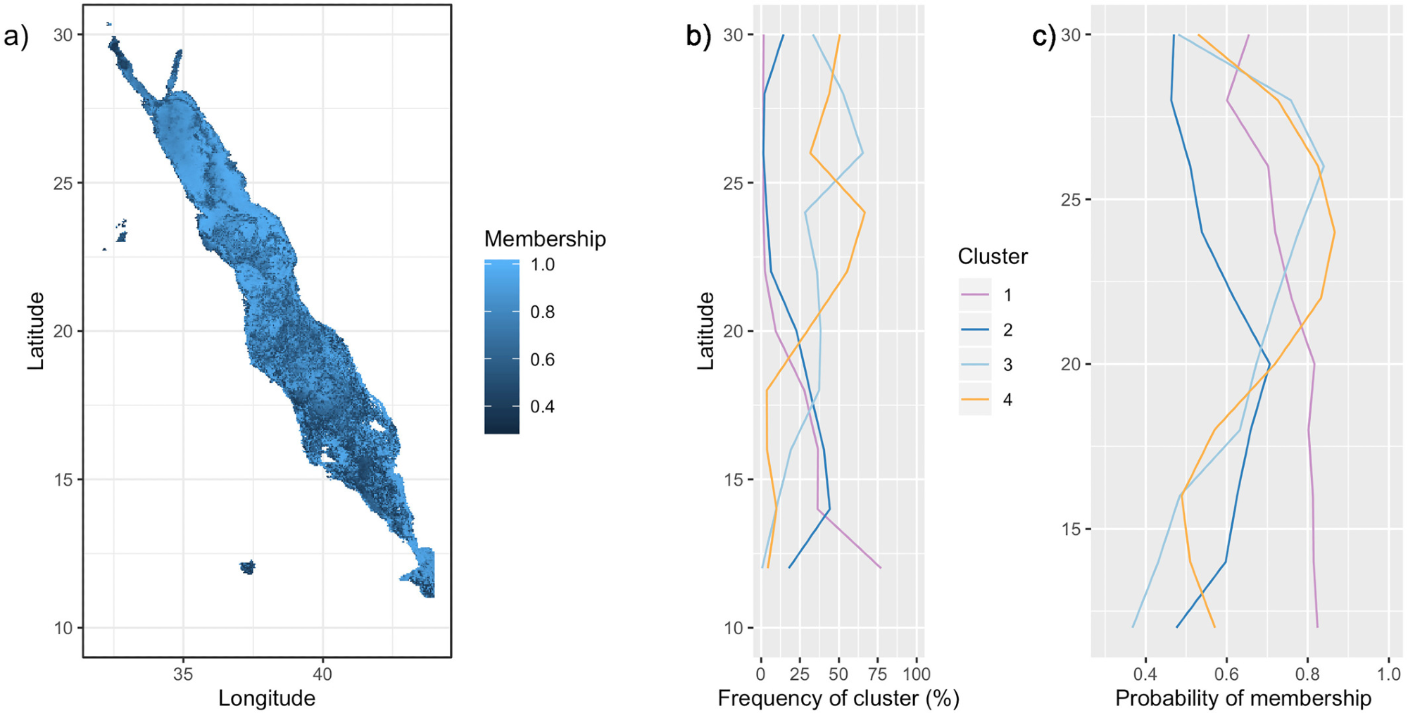
Figure 4. Probability of bio-region membership. (a) Probabilities of membership of each pixel to its assigned bio-region. Trend lines on the right depict (b) the frequency of occurrence of each bio-region by latitude, and (c) the average probability of membership by latitude for each bio-region. Latitudinal bands of 2 were used. Image Credit: Kheireddine, et al., 2021
Bio-region 1 had a summer phytoplankton bloom from the end of May and peaked in July, collapsing in August. The bio-region 2 was characterized by a peak in CHL in summer (from the end of May and ceased in September) and in fall-winter (October–February), which might be the consequences of the summer southwest monsoon and the winter northeast monsoon, respectively. The shallow waters and the onshore coastal habitats of the southern Red Sea had higher CHL values compared to the northern bio-regions (see Figures 2a, 2b, and 5), suggesting that the northern half is more oligotrophic.
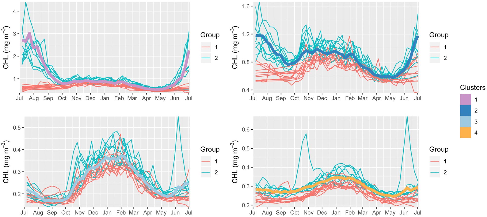
Figure 5. Climatological annual cycles vs. yearly annual cycles. For each bio-region, the climatological annual cycles chlorophyll-a concentration (thick lines) is compared with all 21 annual cycles available (thin lines, from 1998 to 2018). The two groups of years mentioned in “Inter-annual variability in the annual cycle of CHL” within the manuscript and Table 1 are highlighted, Group 1: 1998 to 2001 and 2012 to 2018; Group 2: 2002 to 2011. Image Credit: Kheireddine, et al., 2021
Analysis of the yearly annual cycles revealed two diverse groups of years (see Figure 5 and Table 2) that had distinct CHL annual cycles in Bio-regions 1 and 2 and only small variations in Bio-regions 3 and 4. These differences might be due to the lesser availability of the yearly CHL annual cycle in the Red Sea’s southern part.
Table 2. Years and MEI phase associated to Group 1 and Group 2 highlighted in Figure 5. Source: Kheireddine, et al., 2021
| |
Group 1 |
Group 2 |
| Years |
1998, 1999, 2000, 2001, 2012, 2013, 2014, 2015, 2016, 2017, 2018 |
2002, 2003, 2004, 2005, 2006, 2007, 2008, 2009, 2010, 2011 |
| MEI phase |
Mainly negative (72%) |
Mainly positive (85%) |
Earlier research has indicated that ENSO could influence the global climate and impact the phytoplankton phenology. Positive ENSO phases showed a deeper nutricline, an increase in stratification, and thus a decreased CHL concentration in the ocean.
The research focused on the spatiotemporal and inter-annual variability of the phytoplankton phenology in the basin’s northern part. For this, an annual clustering technique was employed (see Figure 6).
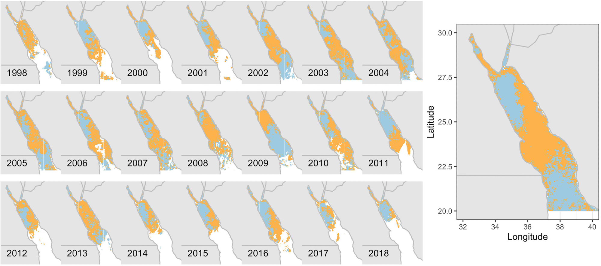
Figure 6. Annual clustering results from the northern part of the Red Sea. (left) Annual spatial distribution of bio-regions #3 and #4 from 1998 to 2018, and (right) the average map. Image Credit: Kheireddine, et al., 2021
Figure 7 illustrates the annual clustering results of Bioregions 3 and 4.
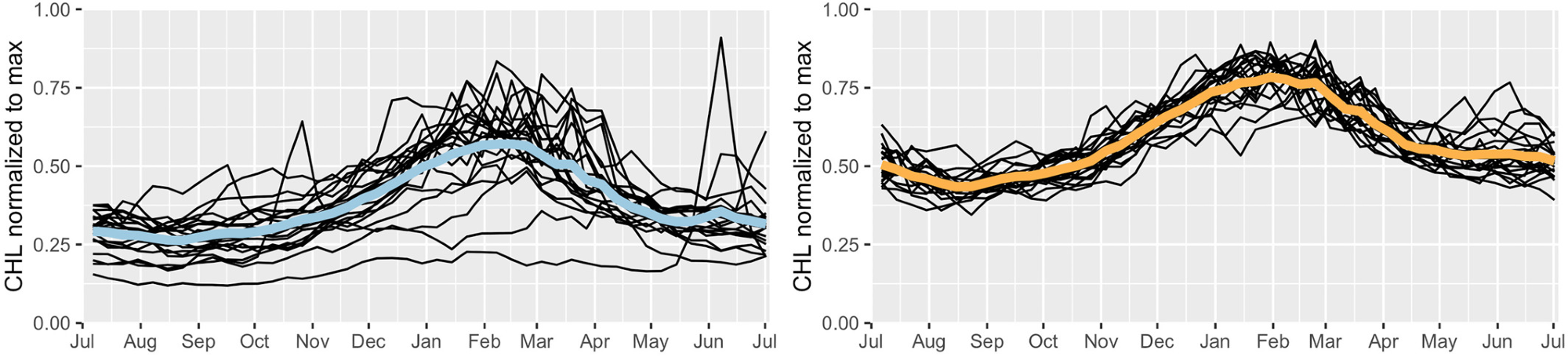
Figure 7. Annual clustering results for the northern half of the Red Sea (above 20°N). The average annual cycles of normalized chlorophyll-a concentration (thick lines) with all annual cycles (thin lines) for bio-regions #3 and #4. Image Credit: Kheireddine, et al., 2021
The annual cycles of CHL from 1998–2018 demonstrated that the Bio-region 3 showed greater variability in the phytoplankton phenology which might be due to the differences in surface circulation, sea surface temperature, and/or mesoscale activity.
The phytoplankton bloom seen majorly in the Bioregion 3 takes place when the mixing is deep enough to provide surface layers with nutrients from deep waters. Figure 8 illustrates the MLD of the northwestern Red Sea from 1998 to 2018.
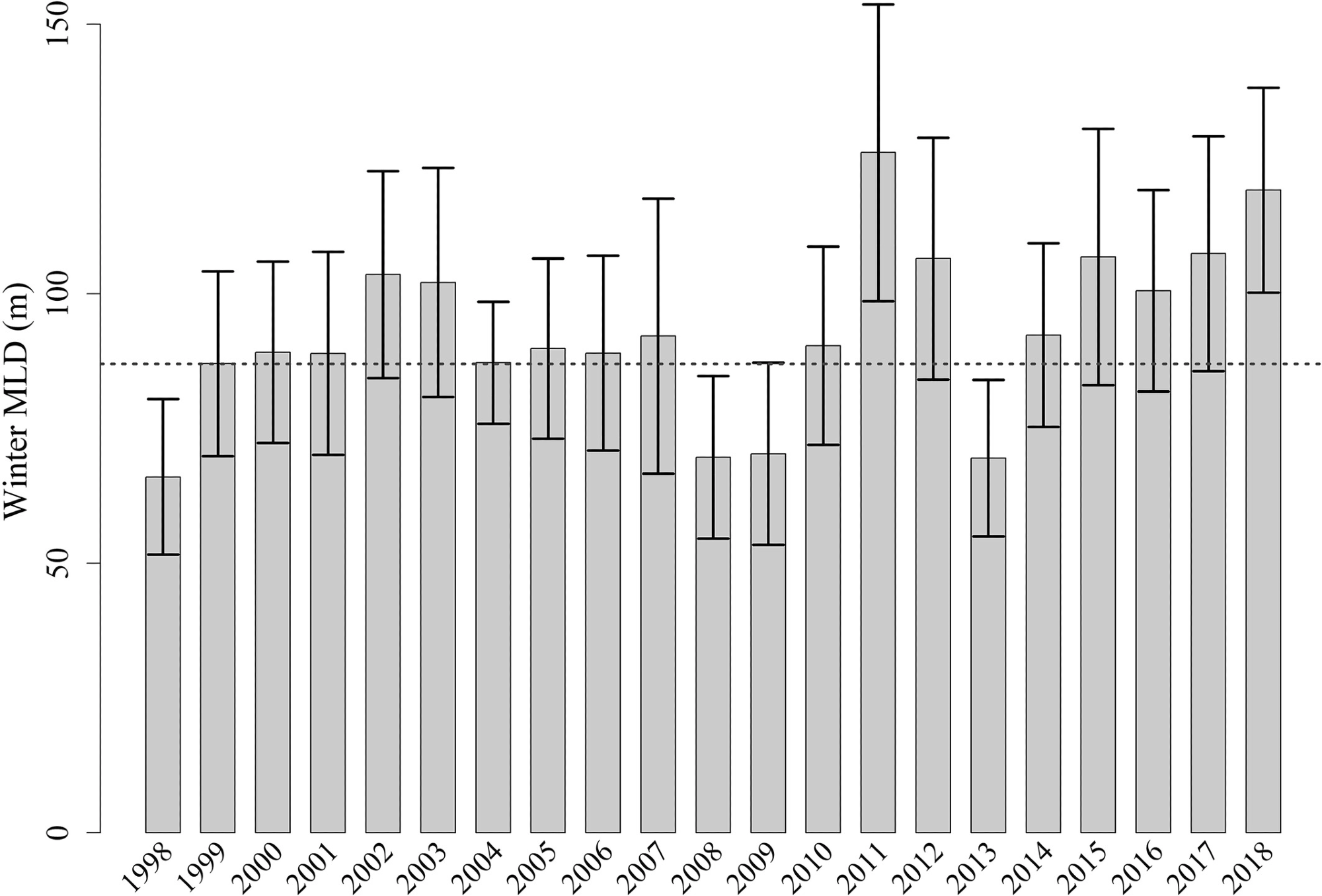
Figure 8. Average ± standard deviation of the winter Mixed Layer Depth within the northwestern Red Sea from 1998 to 2018. The dashed dark gray line represents the average value of the MLD. Image Credit: Kheireddine, et al., 2021
The winter bloom observed in the central part of the Red Sea might be due to the convergence zone developed by opposite surface winds and also from the vertical mixing that distributed phytoplankton from the deep CHL maximum.
Moreover, earlier works revealed that physical-like mesoscale features also supply nutrients to the region which induces phytoplankton growth.
Conclusion
The research revealed the potential of employing ocean color data to analyze phytoplankton phenology. The observations offer a deeper understanding of phytoplankton phenology in the Red Sea. However, in situ measurements are also required for the complete comprehension of the mechanisms that bestow to phytoplankton seasonal cycle in the basin.
Journal Reference:
Kheireddine, M., Mayot, N., Ouhssain, M., Jones, B. H. (2021) Regionalization of the Red Sea Based on Phytoplankton Phenology: A Satellite Analysis. Journal of Geophysical Research: Oceans, 126(10), p. e2021JC017486. Available online: https://agupubs.onlinelibrary.wiley.com/doi/10.1029/2021JC017486.
References and Further Reading
- Acker, J., et al. (2008) Remotely-sensed chlorophyll a observations of the northern Red Sea indicate seasonal variability and influence of coastal reefs. Journal of Marine Systems, 69(3–4), pp. 191–204. doi.org/10.1016/j.jmarsys.2005.12.006.
- Antoine, D., et al. (2006) BOUSSOLE: A joint CNRS-INSU, ESA, CNES and NASA ocean color calibration and validation activity. NASA Technical memorandum N° 2006–214147, pp. 61. NASA/GSFC.
- Ardyna, M., et al. (2014) Recent Arctic Ocean sea ice loss triggers novel fall phytoplankton blooms. Geophysical Research Letters, 41(17), pp. 6207–6212. doi.org/10.1002/2014gl061047.
- Ardyna, M., et al. (2017) Delineating environmental control of phytoplankton biomass and phenology in the Southern Ocean. Geophysical Research Letters, 44(10), pp. 5016–5024. doi.org/10.1002/2016gl072428.
- Asfahani, K., et al. (2020) Capturing a mode of intermediate water formation in the Red Sea. Journal of Geophysical Research-Oceans, 125(4). doi.org/10.1029/2019jc015803.
- Baars, M., et al. (1998) Seasonal fluctuations in plankton biomass and productivity in the ecosystems of the Somali Current, Gulf of Aden, and Southern Red Sea. In: Sherman, K., et al. (Eds); Large marine ecosystems of the Indian Ocean: Assessment, sustainability, and management. Blackwell Science, Inc., pp. 394.
- Behrenfeld, M J & Boss, E S (2018). Student’s tutorial on bloom hypotheses in the context of phytoplankton annual cycles. Global Change Biology, 24(1), pp. 55–77.
- Behrenfeld, M. J., et al. (2006). Climate-driven trends in contemporary ocean productivity. Nature, p. 444. doi.org/10.1038/nature05317.
- Bopp, L & Le Quéré, C (2009). Ocean carbon cycle. In: Le Quéré, C (Ed.), Surface ocean—lower atmosphere processes, geophysical monograph series, (Vol. 187, pp. 181–195). American Geophysical Union. doi.org/10.1029/2008gm000780.
- Boyce, D. G., et al. (2017) Environmental structuring of marine plankton phenology. Nature Ecology & Evolution, 1(10), pp. 1484–1494. doi.org/10.1038/s41559-017-0287-3.
- Boyd, P. W., et al. (2019) Multi-faceted particle pumps drive carbon sequestration in the ocean. Nature, 568(7752), pp. 327–335. doi.org/10.1038/s41586-019-1098-2.
- Brewin, R. J. W., et al. (2015) Regional ocean-color chlorophyll algorithms for the Red Sea. Remote Sensing of Environment, 165, pp. 64–85. doi.org/10.1016/j.rse.2015.04.024.
- Chaidez, V., et al. (2017) Decadal trends in Red Sea maximum surface temperature. Scientific Reports, 7. doi.org/10.1038/s41598-017-08146-z.
- Chavez, F. P., et al. (2011) Marine primary production in relation to climate variability and change. In: Carlson, C A & Giovannoni S J (Eds), Marine primary production in relation to climate variability and change. Annual review of marine science, 3, pp. 227–260. doi.org/10.1146/annurev.marine.010908.163917.
- Churchill, J. H., et al. (2014) The transport of nutrient-rich Indian Ocean water through the Red Sea and into coastal reef systems. Journal of Marine Research, 72(3), pp. 165–181.
- Cushing, D. H., et al. (1990). Plankton production and year-class strength in fish populations - An update of the match mismatch hypothesis. Advances in Marine Biology, 26, pp. 249–293. doi.org/10.1016/s0065-2881(08)60202-3.
- Dall’Olmo, G., et al. (2016) Substantial energy input to the mesopelagic ecosystem from the seasonal mixed-layer pump. Nature Geoscience, 9(11), pp. 820–823. doi.org/10.1038/ngeo2818.
- Dasari, H. P., et al. (2018) ENSO influence on the interannual variability of the Red Sea convergence zone and associated rainfall. International Journal of Climatology, 38(2), pp. 761–775. doi.org/10.1002/joc.5208.
- de Boyer Montégut, C., et al. (2004) Mixed layer depth over the global ocean: An examination of profile data and a profile-based climatology. Journal of Geophysical Research, 109(12), pp. 1–20. doi.org/10.1029/2004JC002378.
- D'Ortenzio, F., et al. (2012) Phenological changes of oceanic phytoplankton in the 1980s and 2000s as revealed by remotely sensed ocean-color observations. Global Biogeochemical Cycles, 26. doi.org/10.1029/2011gb004269.
- D'Ortenzio, F & d’Alcala, M R (2009) On the trophic regimes of the Mediterranean Sea: A satellite analysis. Biogeosciences, 6(2), pp. 139–148. doi.org/10.5194/bg-6-139-2009.
- Dreano, D., et al. (2016) The Gulf of Aden intermediate water intrusion regulates the southern Red Sea summer phytoplankton blooms. PLoS ONE, 11(12), p. e0168440. doi.org/10.1371/journal.pone.0168440.
- Edwards, M & Richardson, A J (2004) Impact of climate change on marine pelagic phenology and trophic mismatch. Nature, 430(7002), pp. 881–884. doi.org/10.1038/nature02808.
- Eladawy, A., et al. (2017) Characterization of the northern Red Sea’s oceanic features with remote sensing data and outputs from a global circulation model. Oceanologia, 59(3), pp. 213–237. doi.org/10.1016/j.oceano.2017.01.002.
- Genevier, L. G. C., et al. (2019) Marine heatwaves reveal coral reef zones susceptible to bleaching in the Red Sea. Global Change Biology, 25(7), pp. 2338–2351. doi.org/10.1111/gcb.14652.
- Gittings, J. A., et al. (2019). Remotely sensing phytoplankton size structure in the Red Sea. Remote Sensing of Environment, 234, p. 111387. doi.org/10.1016/j.rse.2019.111387.
- Gittings, J. A., et al. (2019) Evaluating tropical phytoplankton phenology metrics using contemporary tools. Scientific Reports, p. 9. doi.org/10.1038/s41598-018-37370-4.
- Gittings, J. A., et al. (2008) Impacts of warming on phytoplankton abundance and phenology in a typical tropical marine ecosystem. Scientific Reports, 8. doi.org/10.1038/s41598-018-20560-5.
- Karnauskas, K B & Jones, B H (2018) The interannual variability of sea surface temperature in the Red Sea from 35 years of satellite and in situ observations. Journal of Geophysical Research: Oceans, 123, pp. 5824–5841. doi.org/10.1029/2017JC013320.
- Kheireddine, M., et al. (2020) Organic carbon export and loss rates in the Red Sea. Global Biogeochemical Cycles, 34(10). doi.org/10.1029/2020gb006650.
- Kheireddine, M., et al. (2017) Assessing pigment-based phytoplankton community distributions in the Red Sea. Frontiers in Marine Science, 4. doi.org/10.3389/fmars.2017.00132.
- Kheireddine, M., et al. (2018) Light absorption by suspended particles in the Red Sea: Effect of phytoplankton community size structure and pigment composition. Journal of Geophysical Research-Oceans, 123(2), pp. 902–921. doi.org/10.1002/2017jc013279.
- Koeller, P., et al. (2009) Basin-scale coherence in phenology of shrimps and phytoplankton in the North Atlantic Ocean. Science, 324(5928), pp. 791–793. doi.org/10.1126/science.1170987.
- Labiosa, R. G., et al. (2003) The interplay between upwelling and deep convective mixing in determining the seasonal phytoplankton dynamics in the gulf of Aqaba: Evidence from SeaWiFS and MODIS. Limnology & Oceanography, 48, pp. 2355–2368.
- Lacour, L., et al. (2015) Phytoplankton biomass cycles in the North Atlantic subpolar gyre: A similar mechanism for two different blooms in the Labrador Sea. Geophysical Research Letters, 42(13), pp. 5403–5410. doi.org/10.1002/2015gl064540.
- Langodan, S., et al. (2014) The Red Sea: A natural laboratory for wind and wave modeling. Journal of Physical Oceanography, 44(12), pp. 3139–3159. doi.org/10.1175/jpo-d-13-0242.1.
- Lindel, D & Post, A (1995) Ultraphytoplankton succession is triggered by deep winter mixing in the Gulf of Aqaba (Eilat), Red Sea. Limnology & Oceanography, 40(6), pp. 1130–1141. doi.org/10.4319/lo.1995.40.6.1130.
- Martinez, E., et al. (2009) Climate-Driven Basin-Scale decadal oscillations of oceanic phytoplankton. Science, 326(5957), pp. 1253–1256. doi.org/10.1126/science.1177012.
- Mayot, N., et al. (2016) Interannual variability of the Mediterranean trophic regimes from ocean color satellites. Biogeosciences, 13(6), pp. 1901–1917. doi.org/10.5194/bg-13-1901-2016.
- Morcos, S A (1970) Physical and chemical oceanography of the Red Sea. Oceanography and Marine Biology: An Annual Review, 8, pp. 73–202.
- Papadopoulos, V. P., et al. (2013) Atmospheric forcing of the winter air-sea heat fluxes over the Northern Red Sea. Journal of Climate, 26 (5), pp. 1685–1701. doi.org/10.1175/jcli-d-12-00267.1.
- Papadopoulos, V. P., et al. (2015) Factors governing the deep ventilation of the Red Sea. Journal of Geophysical Research-Oceans, 120 (11), pp. 7493–7505. doi.org/10.1002/2015jc010996.
- Platt, T., et al. (2003) Spring algal bloom and larval fish survival. Nature, 423(6938), pp. 398–399. doi.org/10.1038/423398b.
- Racault, M. F., et al. (2012) Phytoplankton phenology in the global ocean. Ecological Indicators, 14(1), pp. 152–163. doi.org/10.1016/j.ecolind.2011.07.010.
- Racault, M. F., et al. (2015) Phytoplankton phenology indices in coral reef ecosystems: Application to ocean-color observations in the Red Sea. Remote Sensing of Environment, 160, pp. 222–234. doi.org/10.1016/j.rse.2015.01.019.
- Racault, M. F., et al. (2017) Impact of El Nino variability on oceanic phytoplankton. Frontiers in Marine Science, 4. doi.org/10.3389/fmars.2017.00133.
- Racault, M. F., et al. (2017) Phenological responses to ENSO in the global oceans. Surveys in Geophysics, 38(1), pp. 277–293. doi.org/10.1007/s10712-016-9391-1.
- Racault, M.-F., et al. (2014) Impact of missing data on the estimation of ecological indicators from satellite ocean-color time-series. Remote Sensing of Environment, 152, pp. 15–28. doi.org/10.1016/j.rse.2014.05.016.
- Raitsos, D. E., et al. (2013) Remote sensing the phytoplankton seasonal succession of the Red Sea. PLoS ONE, 8(6), pp. e64909. doi.org/10.1371/journal.pone.0064909.
- Raitsos, D. E., et al. (2015) Monsoon oscillations regulate fertility of the Red Sea. Geophysical Research Letters, 42(3), pp. 855–862. doi.org/10.1002/2014gl062882.
- Reid, P C & Beaugrand, G (2012). Global synchrony of an accelerating rise in sea surface temperature. Journal of the Marine Biological Association of the United Kingdom, 92(7), pp. 1435–1450. doi.org/10.1017/s0025315412000549.
- Sathyendranath, S., et al. (2019) An ocean-colour time series for use in climate studies: The experience of the Ocean-Colour climate change initiative (oC-CCI). Sensors, 19, 4285. doi.org/10.3390/s19194285.
- Sathyendranath, S., et al. (2020) ESA ocean colour climate change initiative (Ocean_Colour_cci): Global chlorophyll-a data products gridded on a sinusoidal projection. Version 4.2, Centre for Environmental Data Analysis. Retrieved. Available at: https://catalogue.ceda.ac.uk/uuid/99348189bd33459cbd597a58c30d8d10.
- Sathyendranath, S., et al. (2015) Revisiting Sverdrup's critical depth hypothesis. ICES Journal of Marine Science, 72(6), pp. 1892–1896. doi.org/10.1093/icesjms/fsv110.
- Sofianos, S S & Johns, W E (2003) An Oceanic General Circulation Model (OGCM) investigation of the Red Sea circulation: 2. Three-dimensional circulation in the Red Sea. Journal of Geophysical Research-Oceans, 108(C3). doi.org/10.1029/2001jc001185.
- Sofianos, S S & Johns, W E (2007) Observations of the summer Red Sea circulation. Journal of Geophysical Research, 112(C6). doi.org/10.1029/2006jc003886.
- Steinberg, D. K., et al. (2001) Overview of the US JGOFS Bermuda Atlantic Time-series Study (BATS): A decade-scale look at ocean biology and biogeochemistry. Deep-Sea Research Part II: Topical Studies in Oceanography, 48, pp. 1405–1447. doi.org/10.1016/s0967-0645(00)00148-x.
- Torfstein, A & Kienast, S S (2018) No correlation between atmospheric dust and surface ocean chlorophyll-a in the oligotrophic Gulf of Aqaba, northern Red Sea. Journal of Geophysical Research: Biogeosciences, 123, pp. 391–405. doi.org/10.1002/2017JG004063.
- Triantafyllou, G., et al. (2014) Exploring the Red Sea seasonal ecosystem functioning using a three-dimensional biophysical model. Journal of Geophysical Research-Oceans, 119(3), pp. 1791–1811. doi.org/10.1002/2013jc009641.
- Wolter, K & Timlin, M S (1993) Monitoring ENSO in COADS with a seasonally adjusted principal component index. In: Proceedings of the 17th climate diagnostics workshop, pp. 52–57. NOAA/NMC/CAC-NSSL-Oklahoma Climate Survey-CIMMS-School of Meteorology of the University of Oklahoma.
- Wolter, K & Timlin, M S (1998) Measuring the strength of ENSO events - How does 1997/98 rank? Weather, 53, pp. 315–324. doi.org/10.1002/j.1477-8696.1998.tb06408.x.
- Wolter, K & Timlin, M S (2011) El Nino/Southern oscillation behaviour since 1871 as diagnosed in an extended multivariate ENSO index (MEI.ext). International Journal of Climatology, 31(7), pp. 1074–1087. doi.org/10.1002/joc.2336.
- Yao, F. C., et al. (2014) Seasonal overturning circulation in the Red Sea: 2. Winter circulation. Journal of Geophysical Research-Oceans, 119(4), pp. 2263–2289. doi.org/10.1002/2013jc009331.
- Yao, F. C., et al. (2014) Seasonal overturning circulation in the Red Sea: 1. Model validation and summer circulation. Journal of Geophysical Research-Oceans, 119(4), pp. 2238–2262. doi.org/10.1002/2013jc009004.
- Zarokanellos, N D & Jones, B H (2021). Influences of physical and biogeochemical variability of the central Red Sea during winter. Journal of Geophysical Research: Oceans, 126, p. e2020JC016714. doi.org/10.1029/2020JC016714.