Plastics are widely used materials in society today, but only a small percentage of consumer plastics are recycled into new products. Plastics’ characteristics and costs favor their use in disposable and single-use products, which unfortunately gather as pollutants in our ecosystems due to poor waste management.
Image Credit: Nenad Nedomacki/Shutterstock.com
In a typical recycling process, plastic waste is reduced in size, for example, by chopping, washing, and then separating using flotation or mechanical sorting. Plastic purities range from 75-95% by mass, but the industrial sector requires plastic purities of 95%.
Henriksen, M. L. et al. analyzed plastics with a hyperspectral camera in the wavelength range of 1000-2500 nm, and the use of a hierarchical model helped identify individual plastic types.
This study determined whether detailed plastic-type recognition is possible utilizing reflection imaging using a hyperspectral camera (HC) technology in the wavelength range of 955-1700 nm with minimal data processing—only using normalization and a Savitzky-Golay filter. The spectral data was used to build an unsupervised machine learning model that can differentiate between types of plastic and categorize three unknown plastic samples.
Methodology
The study analyzed 13 commercially available plastics, set out in table 1.
Table 1. Plastic identification, plastic type, trade name, supplier for the materials included in this study. Source: Henriksen, et al., 2022
| ID |
Plastic type |
Name |
Supplier |
| HDPE |
Polyethylene |
PE 100 |
SIMONA |
| PP |
Polypropylene |
240-CA12 |
INEOS |
| PS |
Polystyrene |
CD cover |
– |
| PVC |
Poly(vinyl chloride) |
PVC-U |
GEHR |
| PVDF |
Poly(vinylidene difluoride) |
PVDF |
GEHR |
| POM N |
Polyoxymethylene |
Ertacetal C |
Mitsubishi |
| POM B |
Polyoxymethylene |
Ertacetal C |
Mitsubishi |
| PEEK |
Polyetheretherketone |
Ketron PEEK 1000 |
Mitsubishi |
| ABS |
Poly(acrylonitrile-butadiene-styrene) |
Terluran GP35 |
INEOS |
| PMMA |
Poly(methyl methacrylate) |
Setacryl 1000 |
Madreperla |
| PC |
Polycarbonate |
Makrolon 2652 |
Covestro |
| PET |
Poly(ethylene therphalate) |
CB-602 |
UltraPurge |
| PA12 |
Polyamide 12 |
PA 12-TR |
GEHR |
| U1 |
Unknown |
Weighing boat (White) |
VWR |
| U2 |
Unknown |
Plexiglas |
Rias |
| U3 |
Unknown |
Safety glasses |
VWR |
The disks’ and unknown samples’ Fourier transformed infrared (FT-IR) spectra were gathered in an attenuated total reflection (ATR) mode on an iS5 spectrophotometer fitted with a ZnSe crystal.
Prior to measurement, a sample of 5–10 mg was cut from the sample discs and locked into aluminum pans. Samples of 5–10 mg are heated in a TG 209 F1 Libra from 35 °C to 800 °C at a rate of 10 °C min-1 in both laboratory air and nitrogen.
The hyperspectral camera (HC) setup is operated in its own space to reduce the impact of changing temperature, light, and humidity. In a typical experiment, the samples were loaded onto the conveyer belt and all lights, except the halogen lamps, were turned off. The samples were passed by the scan line at a speed of 3.75 m min-1 before being transferred to a laptop computer.
The spectra are documented as in 2.6.1, with the exceptions of 1) being kept as reflectance and 2) being cropped to 972–1675 nm. The loading matrix was extracted and used to post-process the unknown sample spectra, as shown in Table 1 by U1, U2, and U3.
Results and Discussion
Figure 1 shows the stacked FT-IR spectra of all materials.
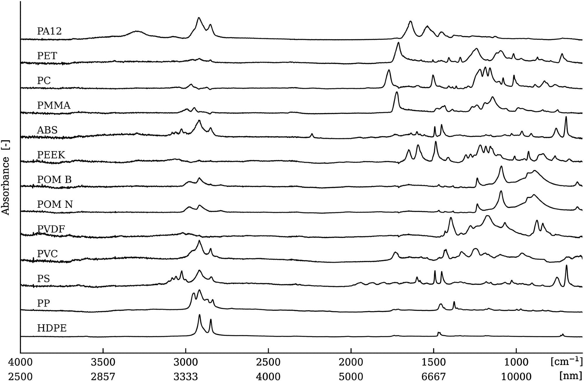
Figure 1. FT-IR spectra for the materials tested. The spectra are shifted for visual clarity. Image Credit: Henriksen, et al., 2022
Table 2 shows melting temperature (Tm), glass transition temperature (Tg), and decomposition temperature (Td) determined in DSC and TGA.
Table 2. Glass transition temperature (Tg), melting temperature (Tm), and decomposition temperature (Td) for the materials analyzed by differential scanning calorimetry (DSC) and thermogravimetrical analysis (TGA). TGA data is given as the Td (mass loss%). Source: Henriksen, et al., 2022
| |
Tg [°C]α |
Tm [°C]α |
Td [°C]β |
Td [°C]γ |
| HDPE |
– |
138 |
427 (100) |
473 (100) |
| PP |
– |
149 |
328 (100) |
458 (100) |
| PS |
101 |
– |
367 (100) |
415 (98) |
| PVC |
82 |
– |
284 (59) 433 (36) |
292 (59) 468 (23) |
| PVDF |
– |
172 |
404 (57) 558 (41) |
452 (68) |
| POM N |
– |
169 |
285 (94) |
355 (99) |
| POM B |
– |
170 |
313 (100) |
357 (100) |
| PEEK |
– |
341 |
580 (31) 661 (94) |
592 (45) |
| ABS |
110 |
– |
411 (92) 552 (8) |
428 (93) |
| PMMA |
129 |
– |
317 (98) |
374 (99) |
| PC |
149 |
– |
506 (73) 618 (100) |
513 (80) |
| PET |
86 |
250 |
428 (85) 574 (100) |
438 (84) |
| PA12 |
159 |
– |
420 (93) 535 (100) |
437 (98) |
α DSC at 20 °C min−1.
β TGA at 20 °C min−1 in air.
γ TGA at 20 °C min−1 in N2.
The thermal properties in Table 2 show that the applied polymers contain little to no additives such as softeners, fillers, and so on. The materials are analyzed using an industrial HC setup, and Figure 2 shows the HC image of four discs at 1204 nm as well as the POM N spectra.
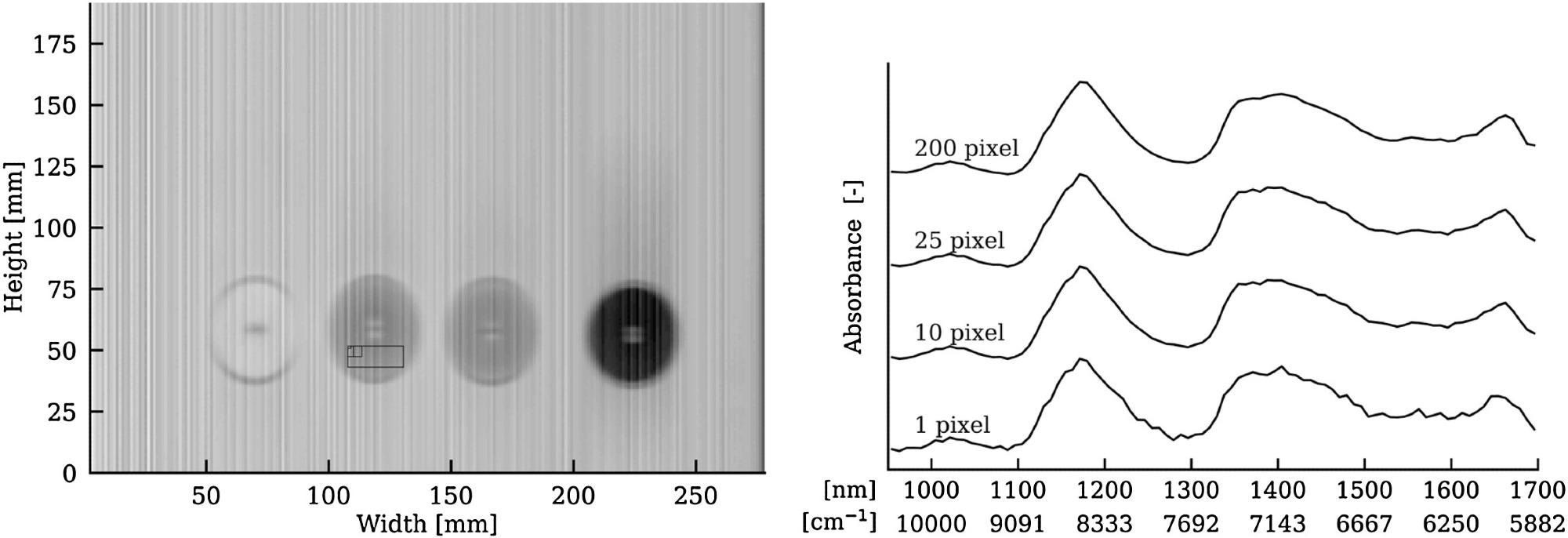
Figure 2. Left, four disks (left to right: PEEK, POM N, POM N, and POM B) presented at 1204 nm and POM N (marked with the area of averaging). Right, hyperspectral spectrum of POM N from scans averaged over 1, 10, 25, and 200 pixels, respectively. Image Credit: Henriksen, et al., 2022
Figure 2 depicts an HC image of four sample discs and the area over which spectral averaging is performed. Figure 3 depicts the spectra of ten ABS discs that were imaged sequentially.
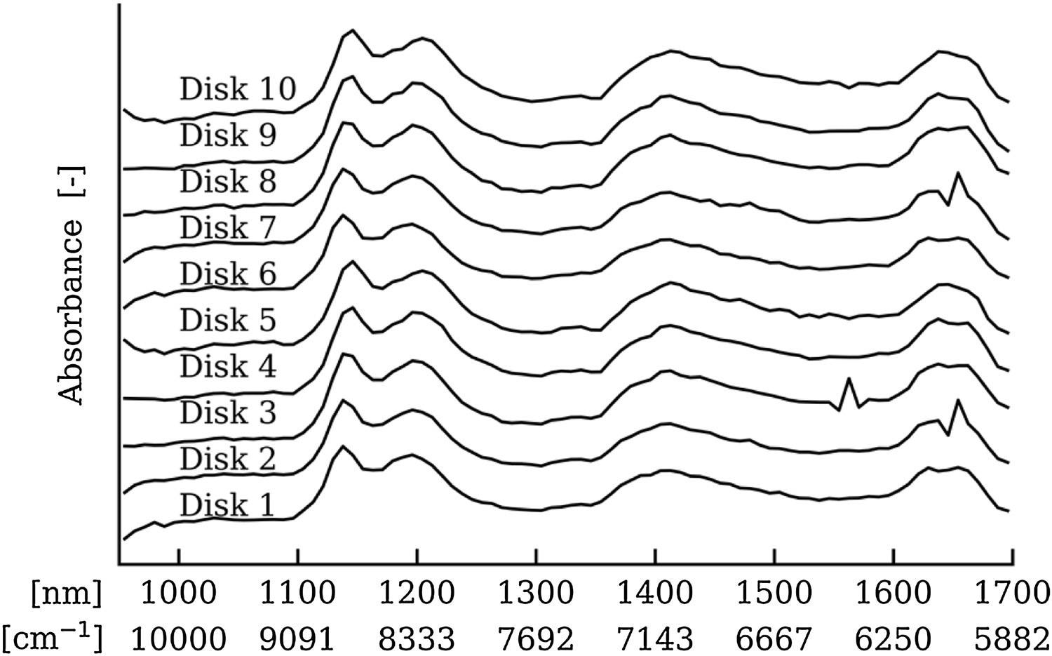
Figure 3. Shows the spectra measured on ten different ABS specimens, each spectrum is an average of 200 pixels. Image Credit: Henriksen, et al., 2022
Figure 3 shows that the spectral data for the ten ABS samples is highly reproducible. Figure 4 depicts the HC spectra obtained from discs with modified surfaces.
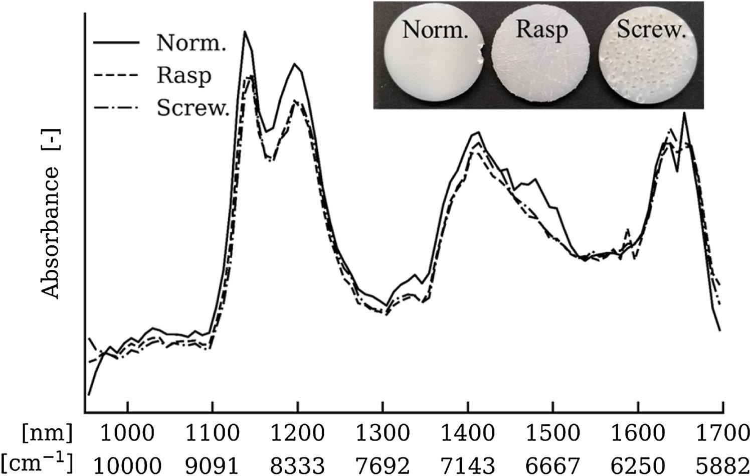
Figure 4. Average spectra measured 10 ABS samples (Norm.), five ABS samples surface treated with a wood rasp (Rasp), and five ABS samples surface treated with screwdriver indentations. Image Credit: Henriksen, et al., 2022
The spectra of all 13 materials in Table 1 were obtained using industrial HC imaging, and the results are shown in Figure 5. Figure 6 shows a PCA score plot on the obtained spectra after Savitzky-Golay filtering.
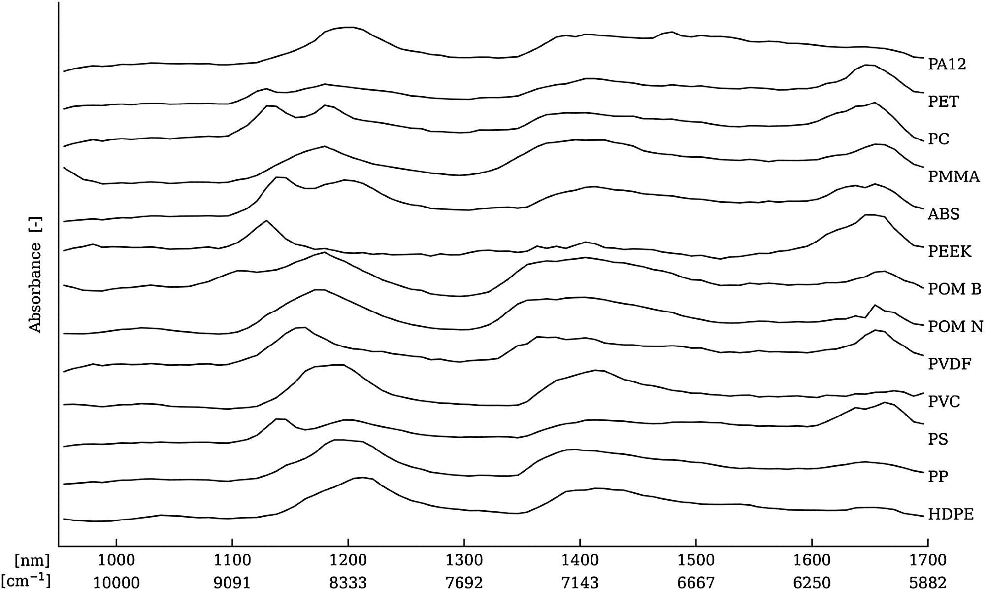
Figure 5. Hyperspectral spectra for all materials averaged over 200 pixels and shifted for visual clarity. Image Credit: Henriksen, et al., 2022
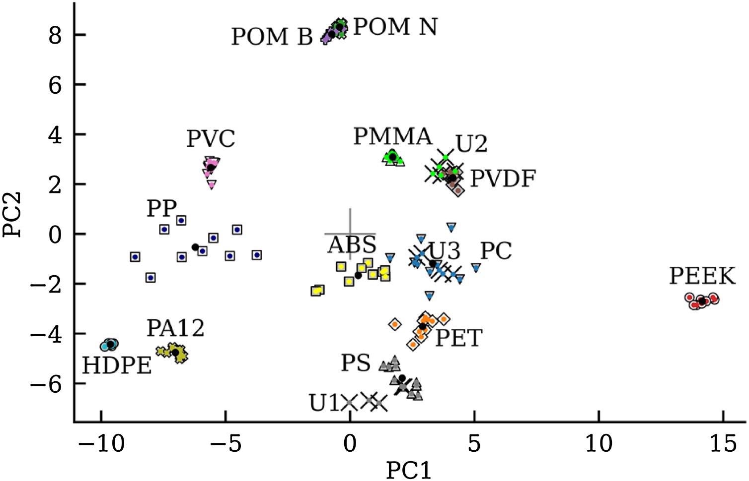
Figure 6. Score plot of the first and second principal component (PC1 and PC2, respectively) from the principal component analysis made on the Savitzky-Golay filtered HC spectra. Calculated cluster centers (black circle), the unknown samples (X), symbols are the known material type, and a color is assigned to the predicted material type. Image Credit: Henriksen, et al., 2022
Figure 6’s score plot shows that the plastic types cluster with good separation.
Since this study is based on industrially available materials that may contain a wide range of additives, material verification was required. The results indicated that the included materials contain low or insignificant concentrations of organic additives.
The spectral quality as a function of surface texture and roughness was studied, and it was discovered that despite a reduction in overall intensity, presumably due to light scattering, the spectral information remained intact as shown in Figure 4.
The majority of the plastics examined are pure, but POM was added as both neutral and blue POM (Table 1 and Figure 5). The PCA (Figure 6) demonstrates that POM formed a dense cluster that was independent of color.
The PCA score-plots revealed that normalization and Savitzky-Golay filtering significantly improved polymer type grouping when compared to raw spectra analysis.
The close grouping of PS, PC, and ABS, on the other hand, increases the uncertainties in differentiating these plastic types.
The unidentified samples (U1, U2, and U3) were randomly chosen in the lab and imaged after the machine learning model was created, about a month after the reference plastics were calculated. The PCA of the unknown samples reveals that U1 is PS, U2 is PMMA, and U3 is PC.
Furthermore, the industrial potential is clearly illustrated because all samples are mapped on a running conveyer belt with an industrial spectrograph, data processing is reduced to a minimum, and machine learning demonstrates its strong predictive power to differentiate between types of plastic.
Conclusion
Hyperspectral imaging with wavelengths ranging from 955-1700 nm on 13 different plastics analyzed by PCA demonstrated that the spectral range is sufficient to distinguish plastics. Unsupervised machine learning has been shown to cluster plastic types, and the resulting loading matrix accurately classified unknown plastic samples.
Since all hyperspectral imaging is carried out with an industrially available spectrograph and with minimal data processing, it is possible to conclude that this evolving technology is the best tool for addressing recycled plastic purity and, thus, the global plastic challenge.
Journal Reference:
Henriksen, M. L., Karlsen, C. B., Klarskov, P., Hinge, M. (2022) Plastic classification via in-line hyperspectral camera analysis and unsupervised machine learning. Vibrational Spectroscopy, 118, p. 103329. Available Online: https://www.sciencedirect.com/science/article/pii/S0924203121001247?via%3Dihub.
References and Further Reading
- Auken, I (2013) Danmark uden affald, Miljø- Og Fødevareministeriet. 14, pp. 1–40.
- Besenbacher, F (2017) Advisory Board for cirkulær økonomi - Anbefalinger til regeringen, Miljø- Og Fødevareministeriet. pp. 1–64.
- Leone, G (2017) The New Plastics Economy: Rethinking the Future of Plastics & Catalysing Action.
- Veltze, S A (2019) Hirsbak, Miljøets fodspor nr. 5 - Affald, Miljøstyrelsen, pp. 1–36.
- Barnes, D K A (2010) Macroplastics at sea around Antarctica, Marine Environmental Research, 70, pp. 250–252. doi.org/10.1016/j.marenvres.2010.05.006.
- Colferai, A. S., et al. (2017) Distribution pattern of anthropogenic marine debris along the gastrointestinal tract of green turtles (Chelonia mydas) as implications for rehabilitation. Marine Pollution Bulletin, 119, pp. 231–237. doi.org/10.1016/j.marpolbul.2017.03.053.
- Corcoran, P. L., et al. (2009) Plastics and beaches: a degrading relationship. Marine Pollution Bulletin, 58, pp. 80–84. doi.org/10.1016/j.marpolbul.2008.08.022.
- Martinez, E., et al. (2009) Floating marine debris surface drift: Convergence and accumulation toward the South Pacific subtropical gyre, Marine Pollution Bulletin, 58, pp. 1347–1355. doi.org/10.1016/j.marpolbul.2009.04.022.
- Ryan, P. G., et al. (2009) Monitoring the abundance of plastic debris in the marine environment. Philosophical Transactions of the Royal Society B, Biological Sciences, 364, pp. 1999–2012. doi.org/10.1098/rstb.2008.0207.
- SUSCHEM (2020) Sustainable Plastics Strategy.
- Thompson, R C (2004) Lost at sea: where is all the plastic? Science, 80(304), p. 838. doi.org/10.1126/science.1094559.
- European Commission (2018) A european strategy for plastics in a circular economy.
- McKinsey & Company (2019), The New Plastics Economy, pp. 1–69.
- Tsakona, M & Rucevska I (2020) Baseline report on plastic waste, Basel Convention, pp. 1–61.
- Serranti, S., et al. (2011) Characterization of post-consumer polyolefin wastes by hyperspectral imaging for quality control in recycling processes. Waste Management, 31, pp. 2217–2227, doi.org/10.1016/j.wasman.2011.06.007.
- Bonifazi, G., et al. (2018) A hierarchical classification approach for recognition of low-density (LDPE) and high-density polyethylene (HDPE) in mixed plastic waste based on short-wave infrared (SWIR) hyperspectral imaging, Spectrochimica Acta Part A: Molecular and Biomolecular Spectroscopy, 198, pp. 115–122. doi.org/10.1016/j.saa.2018.03.006.
- Zheng, Y., et al. (2018) A discrimination model in waste plastics sorting using NIR hyperspectral imaging system, Waste Management, 72, pp. 87–98. doi.org/10.1016/j.wasman.2017.10.015.
- Rozenstein, O., et al. (2017) Development of a new approach based on midwave infrared spectroscopy for post-consumer black plastic waste sorting in the recycling industry, Waste Management, 68, pp. 38–44. doi.org/10.1016/j.wasman.2017.07.023.
- Savitzky, A & Golay M J E (1964) Smoothing and differentiation of data by simplified least squares procedures, Analytical Chemistry, 36, pp. 1627–1639. doi.org/10.1021/ac60214a047.
- Socrates, G (2004) Infrared and Raman Characteristic Group Frequencies: Tables and Charts, 3rd edition, John Wiley & Sons.
- Ruxanda, B., et al. (2009) Preparation and characterization of composites comprising modified hardwood and wood polymers/poly (vinyl chloride), BioResources, 4, pp. 1285–1304.
- Jung, M. R., et al. (2018) Validation of ATR FT-IR to identify polymers of plastic marine debris, including those ingested by marine organisms, Marine Pollution Bulletin, 127, pp. 704–716. doi.org/10.1016/j.marpolbul.2017.12.061.
- Stromberg, R. R., et al. (1934) Infrared spectra of thermally degraded poly (Vinyl chloride). Archive of Journal of Research of the National Bureau, 60(2), pp. 147–152.
- Li, Y., et al. (2011) Zhang, Non-isothermal crystallization process of polyoxymethylene studied by two-dimensional correlation infrared spectroscopy, Polymer, 52, pp. 2059–2069. doi.org/10.1016/j.polymer.2011.03.007.
- Diez-Pascual, A. M., et al. (2009) Synthesis and characterization of poly(ether ether ketone) derivatives obtained by carbonyl reduction, Macromolecules, 42, pp. 6885–6892. doi.org/10.1021/ma901208e.
- Bokria, J. G., et al. (2002) Spatial effects in the photodegradation of poly(acrylonitrilebutadiene-styrene): a study by ATR-FTIR, Polymer, 43, pp. 3239–3246. doi.org/10.1016/S0032-3861(02)00152-0.
- Brandrup, J (2003) Polymer Handbook, 4th edition, John Wiley & Sons.
- Workman, J., et al. (2012) Practical Guide and Spectral Atlas for Interpretive NearInfrared Spectroscopy, 2nd edition, CRC Press. doi.org/10.1201/b11894