The Changing Trends in Marine Cold-Spells Between 1982–2020

By Laura ThomsonApr 6 2022

“Marine heatwaves” (MHWs), also defined as discrete and sustained extreme oceanic warm water episodes, have been the subject of numerous recent studies. Such disasters have devastating effects on marine biodiversity and the regional fishing economy.

Image Credit: Rich Carey/Shutterstock.com

Over the last century, MHWs have increased in frequency, duration, and intensity while MCSs have dropped in the same measures across most ocean surfaces. There have also been hotspots for MHWs and coldspots for MCSs highlighted.

Researchers studied MHWs and MCSs, providing key estimates of global trends in these extremes. Comparative disparities in changes in these extremes’ measurements and background statistics, on the other hand, are less well known.

This research compares the discrepancies between MHW and MCS measures, their multi-decadal trends, and how they correlate to sea surface temperature (SST) statistics from 1982 to 2020 (39-year), using a quantitative MHW and MCS methodology. The studies were published in the Geophysical Research Letters journal.

To answer certain questions, researchers look at everyday satellite SST data to see what the averages and trends are in the MHW and MCS measurements. Secondly, a statistical model is used to determine the relative contributions of long-term SST warming and/or SST variance trends to MCS metric trends. Finally, researchers talk about how their findings might affect marine fisheries and environmental conservation.

Methodology

The Optimum Interpolation (OI) SST dataset, version 2.1, from the National Oceanic and Atmospheric Administration (NOAA) was employed to determine MHWs and MCSs and quantify their parameters globally.

Researchers initially estimated the annual properties from the actual SST data at each grid point to compute trends in SST properties. The temporal trends were then calculated using the Theil–Sen (TS) estimator.

MHWs and MCSs are discrete and long-lasting extreme warm and cool water phenomena in the ocean. Temperature exceedances of the seasonally variable 90th percentile criteria for at least 5 days are classified as MHWs.

MCSs are treated in a similar way, but for temperatures below the tenth percentile. Two consecutive MHWs (or MCSs) with an interval of fewer than two days are considered a single uninterrupted MHW. Figure 1 depicts the MHW definition schematically.

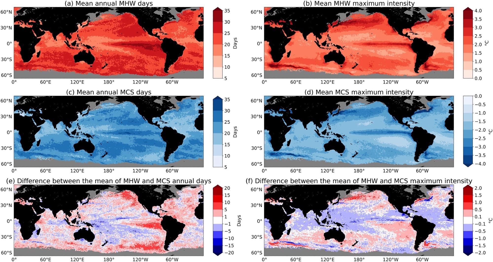
Figure 1. Mean of the marine heatwave (MHW) and marine cold-spells (MCS) annual days and maximum intensity, and the spatial pattern difference between these metrics globally in National Oceanic and Atmospheric Administration Optimum Interpolation sea surface temperature over 1982–2020. Shown are the global pattern of (a) mean annual MHW days, (b) mean MHW maximum intensity, (c) mean annual MCS days, (d) mean MCS maximum intensity, (e) the difference between mean annual MHW days and mean annual MCS days (i.e., (a) mean annual MHW days minus (c) mean annual MCS days), and (f) the difference between the mean MHW maximum intensity and mean MCS maximum intensity (i.e., (b) mean MHW maximum intensity plus (d) mean MCS maximum intensity). For the difference subplots (i.e., (e), (f)), positive values (red regions) represent the annual MHW days as being greater than annual MCS days, MHW maximum intensities are more intense than MCS maximum intensities. Conversely, negative values (blue regions) represent the annual MCS days as being larger than annual MHW days, MCS maximum intensities are more intense than MHW maximum intensities. Image Credit: Wang, et al., 2022

Researchers looked at two MHW and MCS metrics: annual days and maximum intensity. The overall number of MHW (or MCS) days in a year is called annual MHW (or MCS) days. Rather than the peak SST anomaly throughout each single event length, the maximum intensity is characterized as the biggest magnitude SST anomaly appearing within all MHWs or MCSs each year.

A first-order autoregressive (AR1) model was used to produce 500 synthetic SST time series with each OISST grid point, based on the obtained local autoregressive time scale and stochastic variance.

The detected local linear SST trend was added to each of the 500 realizations, and then the MCS metrics (annual days and maximum intensity) and their trends were calculated. If the middle range of 95% of trends in MCS days, for instance, did not span zero, it was thought that mean warming might explain the local trend in MCS days.

If the center range of 95% of trends in MCS measurements did not cross zero, it was considered that the SST variance trend could describe the trend in that metric. Both the SST trend and the SST variance trend can describe the trend in a specific MCS metric.

Results and Discussion

Researchers calculated the mean of the MHW and MCS metrics—annual days and maximum intensity—as a comparative analysis, and then the spatial pattern disparity between these metrics (Figure 1). The mean of MHW and MCS annual days has large regional variability (Figures 1a and 1c), however, they are not symmetric (Figure 1e). In locations of high SST fluctuation, both zones with large maximum MHW and MCS intensity (Figures 1b and 1d) are visible.

The average global MHW/MCS days and maximum intensity time series show clear trends (Figure 2a,2b). From 1982 to 2020, the global average trend in annual MHW days grew by 8.4 days each decade.

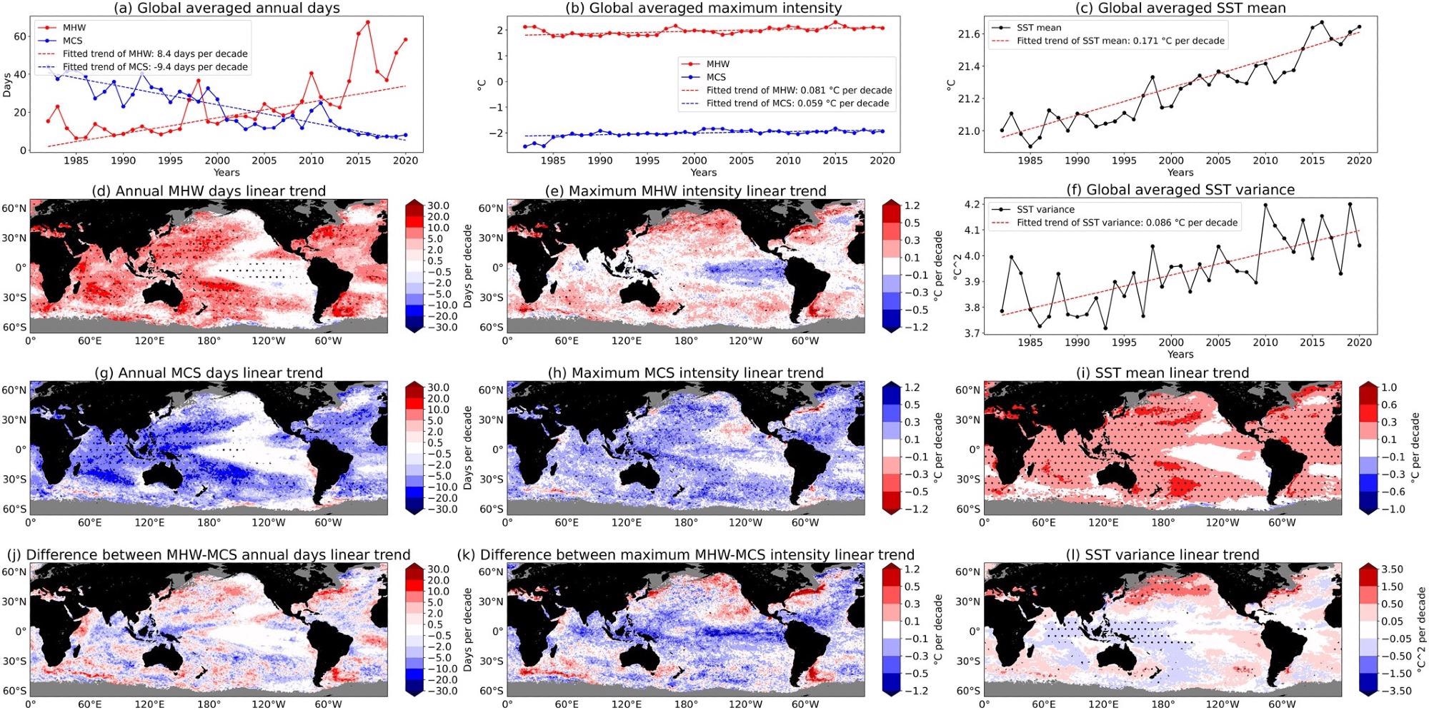
Figure 2. Trends in marine heatwaves (MHW) and marine cold-spells (MCS) metrics as well as sea surface temperature (SST) properties in National Oceanic and Atmospheric Administration Optimal Interpretation SST over 1982–2020. (a), (d), (g), (j) trends in MHW/MCS annual days, (b), (e), (h), (k) trends in maximum MHW/MCS intensity, and (c), (f), (i), (l) trends in SST properties. Shown are globally averaged annual mean time series of (a) MHW and MCS annual days, (b) maximum MHW and MCS intensity, (c) mean SST, and (f) SST variance, as well as the spatial pattern of trends in (d) annual MHW days, (e) maximum MHW intensity, (g) annual MCS days, (h) maximum MCS intensity, (i) SST and (l) SST variance. (j) The spatial pattern of difference between MHW and MCS annual days’ trends (i.e., trends in (d) MHW days plus (g) MCS days). (k) The spatial pattern of difference between maximum MHW and MCS intensity trends (i.e., trends in (e) maximum MHW intensity minus (h) maximum MCS intensity). In (d), (e), (g), (h), all dot hatching areas are where trends are statistically significant at the 95% level. For the difference subplots (i.e., (j), (k)), positive values (red regions) represent MHW days increasing faster than MCS days decreasing, and maximum MHW intensities strengthening faster than maximum MCS intensities weakening. Negative values (blue regions) represent those locations where MCS days decrease faster than MHW days increases, and MCS maximum intensities weaken faster than MHW maximum intensities strengthen. Image Credit: Wang, et al., 2022

El Nio-Southern Oscillation (ENSO) events appear to be associated with the time series of globally averaged yearly MHW/MCS days (Figure 2a). Furthermore, there is no evident ENSO signal in the global mean MHW/MCS maximum intensity time series (Figure 2b).

The global mean annual SST trend is 0.171 °C per decade (Figure 2c), which is double the maximum MHW intensity trend and nearly triple the MCS intensity trend. Absolute SST variance is also growing globally, at a rate of 0.086 °C² every decade (Figure 2f). This corresponds to a 0.022 °C per decade increase in SST standard deviation.

The annual days and maximum intensity of MHW/MCS show significant regional variations across the world (Figures 2d, 2e, 2g, and 2h). From 1982 to 2020, annual MHW days rose in most global oceans (Figure 2d), with certain locations exhibiting increases of more than 20 days each decade.

MCS days, on the other hand, have declined across a broad area of the global ocean (Figure 2g), following the usual spatial pattern of MHW days (cf. Figure 2d). MCS days, on the other hand, have increased as SST has decreased.

The maximum MHW intensity has risen over most of the world’s oceans (Figure 2e), although it has dropped in some areas. Maximum MCS intensities, on the other hand, have diminished in most places (Figure 2h).

The patterns of MHW and MCS trends, as well as SST trends, show an Interdecadal Pacific Oscillation (IPO)-like pattern (Figure 2i).

Variations in annual days and maximum intensity between MHW and MCS are also shown (Figures 2j and 2k). Figure 2j shows how the spatial difference pattern of MHW and MCS annual days varies by region, whereas Figure 2k shows how the pattern of difference in intensity trends varies by region.

Along with SST trends, SST variance trends (Figure 2l) are also shown (Figure 2i). There is a substantial correlation between the SST variance trend (Figure 2l) and the distinct patterns between maximum MHW and MCS intensity trends around the Indo-Pacific warm pool, the North Pacific, the Southern Indian Ocean, and the North and South Atlantic (Figure 2k).

The extensive regional alignment of SST trends (Figure 2i) with MHW and MCS annual days and intensities (Figures 2d, e, g, h) suggests that SST mean warming is mostly responsible for changes in both MHWs and MCSs, but SST variance trends may also play a major role.

Each grid point was investigated to see if the local SST trend, SST variance trend, or both were statistically meaningful drivers of the MCS annual days or maximum intensity trend (Figure 3).

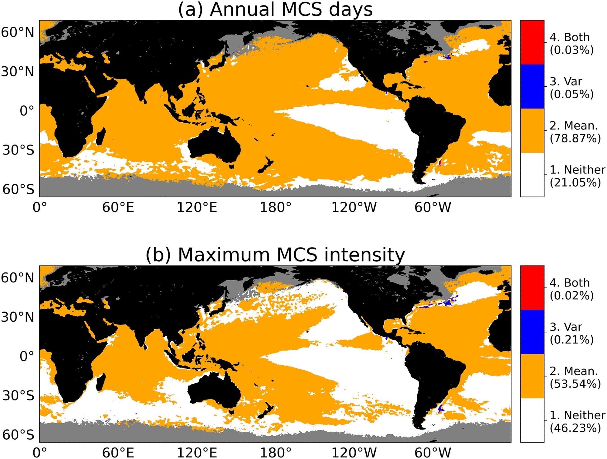
Figure 3. The relative importance of trends in sea surface temperature (SST) and SST variance in driving changes in marine cold spells (MCS) annual days and maximum intensity. Colors indicate whether trends in MCS (a) annual days and (b) maximum intensity are dominated by trends in SST and/or SST variance. Four situation types are shown: ‘neither’ (white), ‘mean-dominant’ (orange), ‘variance-dominant’ (blue), and ‘both’ (red). The proportion of the globe covered by each type is quoted beside in the color bar. Both subplots are derived from National Oceanic and Atmospheric Administration Optimal Interpolation SST from 1982 to 2020. Image Credit: Wang, et al., 2022

Conclusion

The research looked into the changes in average values and trends between MHWs and MCSs, as well as how SST change statistics influenced both measures globally from 1982 to 2020 (39-year).

While the spatial trend patterns in the MHW and MCS measurements are largely comparable, there are some local variances. Variations in maximum intensity trends were shown to be a function of rates of change in SST variability irrespective of baseline, but variations in annual day trends were sensitive to baseline selection.

In different places, the disparities in MHW and MCS intensity trends have changed, and these variations are linked to SST variance changes. As a result, it is indeed critical to know whether the alterations are stable and whether they can be expected to persist.

Future research in this area should focus on determining what causes SST variance variations and whether these changes will persist as the world warms.

In conclusion, researchers discovered that increases in MCS annual days and maximum intensities are dominated by SST trends rather than SST variability trends.

As a result, the research emphasizes the importance of continuing to investigate changes in MHWs/MCSs by taking into account aspects such as multi-decadal variability and whether SST variance would alter over time.

Journal Reference:

Wang, Y., Kajtar, J. B., Alexander, L. V., Pilo, G. S., Holbrook, N. J. (2022) Understanding the Changing Nature of Marine Cold‐Spells. Geophysical Research Letters, 49(6), p. e2021GL097002. Available Online: https://agupubs.onlinelibrary.wiley.com/doi/10.1029/2021GL097002.

References and Further Reading

1. Alexander, M. A., et al. (2018). Projected sea surface temperatures over the 21^st century: Changes in the mean, variability and extremes for large marine ecosystem regions of Northern Oceans. Elementa: Science of the Anthropocene, 6, p. 9. doi.org/10.1525/elementa.191.
2. Banzon, V., et al. (2016). A long-term record of blended satellite and in situ sea-surface temperature for climate monitoring, modeling and environmental studies. Earth System Science Data, 8(1), pp. 165–176. doi.org/10.5194/essd-8-165-2016.
3. Caputi, N., et al. (2016). Management adaptation of invertebrate fisheries to an extreme marine heat wave event at a global warming hot spot. Ecology and Evolution, 6(11), pp. 3583–3593. doi.org/10.1002/ece3.2137.
4. Chen, C & Wang G. (2015). Role of North Pacific mixed layer in the response of SST annual cycle to global warming. Journal of Climate, 28(23), pp. 9451–9458. doi.org/10.1175/JCLI-D-14-00349.1.
5. Chiswell, S M (2021). Atmospheric wavenumber-4 driven South Pacific marine heat waves and marine cool spells. Nature Communications, 12(1), p. 4779. doi.org/10.1038/s41467-021-25160-y.
6. Donders, T. H., et al. (2011). Impact of the Atlantic warm pool on precipitation and temperature in Florida during North Atlantic cold spells. Climate Dynamics, 36(1), pp. 109–118. doi.org/10.1007/s00382-009-0702-9.
7. Dwyer, J. G., et al. (2012). Projected changes in the seasonal cycle of surface temperature. Journal of Climate, 25(18), pp. 6359–6374. doi.org/10.1175/JCLI-D-11-00741.1.
8. Feng, M., et al. (2021). Multi-year marine cold-spells off the west coast of Australia and effects on fisheries. Journal of Marine Systems, 214, p. 103473. doi.org/10.1016/j.jmarsys.2020.103473.
9. Fredston-Hermann, A., et al. (2020). Cold range edges of marine fishes track climate change better than warm edges. Global Change Biology, 26(5), pp. 2908–2922. doi.org/10.1111/gcb.15035.
10. Freitas, C., et al. (2016). Temperature-associated habitat selection in a cold-water marine fish. Journal of Animal Ecology, 85(3), pp. 628–637. doi.org/10.1111/1365-2656.12458.
11. Hare, J. A., et al. (2010). Forecasting the dynamics of a coastal fishery species using a coupled climate - Population model. Ecological Applications, 20(2), pp. 452–464. doi.org/10.1890/08-1863.1.
12. Hobday, A. J., et al. (2016). A hierarchical approach to defining marine heatwaves. Progress in Oceanography, 141, pp. 227–238. doi.org/10.1016/j.pocean.2015.12.014.
13. Holbrook, N. J., et al. (2021). Impacts of marine heatwaves on tropical western and central Pacific Island nations and their communities. Global and Planetary Change, 141, p. 103680. doi.org/10.1016/j.gloplacha.2021.103680.
14. Holbrook, N. J., et al. (2020). Keeping pace with marine heatwaves. Nature Reviews Earth & Environment, 1, pp. 482–493. https://doi.org/10.1038/s43017-020-0068-4.
15. Huang, B., et al. (2021). Improvements of the daily optimum interpolation sea surface temperature (DOISST) version 2.1. Journal of Climate, 34(8), pp. 2923–2939. doi.org/10.1175/JCLI-D-20-0166.1.
16. Jacox, M G (2019). Marine heatwaves in a changing climate. Nature, 571, pp. 485–487. doi.org/10.1038/d41586-019-02196-1.
17. Lirman, D., et al. (2011). Severe 2010 cold-water event caused unprecedented mortality to corals of the Florida reef tract and reversed previous survivorship patterns. PLoS One, 6(8), p. e2307. doi.org/10.1371/journal.pone.0023047.
18. Liu, F., et al. (2020). On the oceanic origin for the enhanced seasonal cycle of SST in the midlatitudes under global warming. Journal of Climate, 33(19), pp. 8401–8413. doi.org/10.1175/JCLI-D-20-0114.1.
19. Morley, J. W., et al. (2017). Marine assemblages respond rapidly to winter climate variability. Global Change Biology, 23(7), pp. 2590–2601. doi.org/10.1111/gcb.13578.
20. Oliver, E C J (2019). Mean warming not variability drives marine heatwave trends. Climate Dynamics, 53, pp. 1653–1659. doi.org/10.1007/s00382-019-04707-2.
21. Oliver, E. C. J., et al. (2021). Marine heatwaves. Annual Review of Marine Science, 13, pp. 313–342. doi.org/10.1146/annurev-marine-032720-095144.
22. Oliver, E. C. J., et al. (2018). Longer and more frequent marine heatwaves over the past century. Nature Communications, 9, p. 1324. https://doi.org/10.1038/s41467-018-03732-9.
23. Pearce, A F & Feng, M (2013). The rise and fall of the “marine heat wave” off Western Australia during the summer of 2010/2011. Journal of Marine Systems, 111–112, pp. 139–156. doi.org/10.1016/j.jmarsys.2012.10.009.
24. Power, S., et al. (1999). Inter-decadal modulation of the impact of ENSO on Australia. Climate Dynamics, 15, pp. 319–324. doi.org/10.1007/s003820050284.
25. Prigent, A., et al. (2020). Origin of weakened interannual sea surface temperature variability in the Southeastern tropical Atlantic Ocean. Geophysical Research Letters, 47(20), p. e2020GL089348. doi.org/10.1029/2020GL089348.
26. Prigent, A., et al. (2020). Weakened SST variability in the tropical Atlantic Ocean since 2000. Climate Dynamics, 54, pp. 2731–2744. doi.org/10.1007/s00382-020-05138-0.
27. Reynolds, R. W., et al. (2007). Daily high-resolution-blended analyses for sea surface temperature. Journal of Climate, 20(22), pp. 5473–5496. doi.org/10.1175/2007JCLI1824.1.
28. Schlegel, R. W., et al. (2021). Marine cold-spells. Progress in Oceanography, 198, p. 102684. doi.org/10.1016/j.pocean.2021.102684.
29. Schlegel, R. W., et al. (2017). Nearshore and offshore co-occurrence of marine heatwaves and cold-spells. Progress in Oceanography, 151, pp. 189–205. doi.org/10.1016/j.pocean.2017.01.004
30. Smale, D. A., et al. (2019). Marine heatwaves threaten global biodiversity and the provision of ecosystem services. Nature Climate Change, 9, pp. 306–312. doi.org/10.1038/s41558-019-0412-1.
31. Smith, K. E., et al. (2021). Socioeconomic impacts of marine heatwaves: Global issues and opportunities. Science, 374(6566), p. eabj3593. doi.org/10.1126/science.abj3593.