Intensification of the Water Cycle Using Satellite-Derived Sea Surface Salinity Measurements

By Laura ThomsonMay 11 2022

Over the ocean, 85% of evaporation (E) and 77% of precipitation (P) happens. Changes in sea surface salinity (SSS) are produced by both processes, resulting in positive (evaporation) and negative (precipitation) abnormalities. The global water cycle is enhanced under a global warming scenario, which is a significant concern due to its deep socioeconomic consequences worldwide. This article will look at recent research published in the Scientific Reports journal.

Image Credit: stockphoto-graf/Shutterstock.com

Since 2000, the Argo system’s worldwide array of temperature and salinity floats and other permanent or regular observation systems have helped advance knowledge of ocean salinity dynamics. SSS observations have been accessible from space since 2010, enhancing the monitoring potential of this Essential Climate Variable.

One of the most significant differences between satellite and in situ salinity measurements is that the latter are generally acquired at a few meters depth (5–10 m), monitoring the near-surface salinity (NSS). In contrast, the former are supplying measurements at the top centimeter layer of the ocean, monitoring the actual SSS.

The vertical stratification of the ocean top levels is responsible for the differences between the SSS and the NSS. The ocean salinity stratification is caused by a complicated mixture of factors, including precipitation, oceanic advection, mixing conditions, freshwater inflow from river runoff, sea ice melt, and evaporation.

The top ocean layer has a roughly uniform density, active vertical mixing, and a high turbulent dissipation rate in the lack of rainfall, continental discharge, or sea ice melting. Vertical salinity gradients in the upper 10 m are likely to be small in this situation.

Researchers show here that the dynamics recorded by satellite SSS measurements are not the same as the dynamics shown by in situ NSS measurements. On the one hand, satellite SSS data show a definite intensification of the water cycle that is not visible in NSS data. Significant variations between SSS and NSS trends, on the other hand, show that global warming is causing increased stratification across large open ocean areas.

Methodology

Researchers utilize the Barcelona Expert Center’s Soil Moisture and Ocean Salinity (SMOS) SSS maps. The BEC SMOS SSS global product v2 comprises a time series of 9-day level 3 salinity maps created daily at a 0.25° × 0.25° grid from 2011 to 2018. In situ salinity data are not used for calibration in the salinity retrieval technique. As a result, the worldwide average of SMOS salinity is set to the global standard of yearly salinity climatology on each map.

The yearly climatological salinity value published by the World Ocean Atlas 2013 (WOA2013) at 0.25° × 0.25° is used as a salinity reference. The average decadal product, which can be found at the National Oceanographic Data Center, is what researchers utilize.

Over the values of Argo measurements, researchers undertake the following quality control: For Argo profiles, the cut-off depth is between 5 and 10 m. Greylist profiles (floats that may have difficulties with one or more sensors) are deleted.

Researchers utilize WOA2013 as a quality indicator: When compared to WOA2013, Argo float profiles with temperature or salinity anomalies of more than 10 °C or 5 psu are eliminated. Only profiles with temperature acquisitions close to the surface between -2.5 and 40 °C and salinity between 2 and 41 psu are used compared to WOA2013.

All remotely sensed surface winds produced from scatterometers and radiometers available are used as observation inputs for the objective approach dealing with the computation of 6-hourly wind fields across the worldwide seas to estimate the 6-hourly blended wind products.

Results

The average salinity at the Argo sites in a 9-day window develops over time over large oceanic regions, such as those between 60° S and 60° N. It is considerably different from the temporal history of the mean salinity in the whole region, as seen in Figure 1.

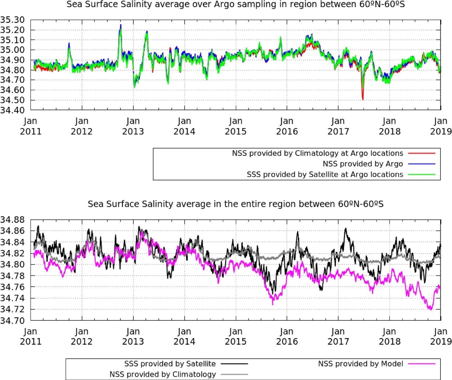
Figure 1. Temporal evolution of the averaged salinity in between 60° S and 60° N. Top plot: The mean salinity measured by Argo floats (blue), the annual climatology averaged at the Argo locations (red), the satellite salinity averaged at the Argo locations (green). Bottom plot: The satellite salinity (black), salinity provided by model (pink) and annual climatology (grey) averaged over the entire region. In the bottom plot the average domain is common and is given by the satellite coverage. The variations in the annual climatology (grey line, bottom plot) correspond to the variations in the satellite coverage that mainly corresponds with the changes in the sea-ice mask. Image Credit: Olmedo, et al., 2022

The maps of averaged salinity for Argo, satellite, and model show comparable geographical trends across the 8-year research period (2011–2018) as shown in the 1st-row Figure 2.

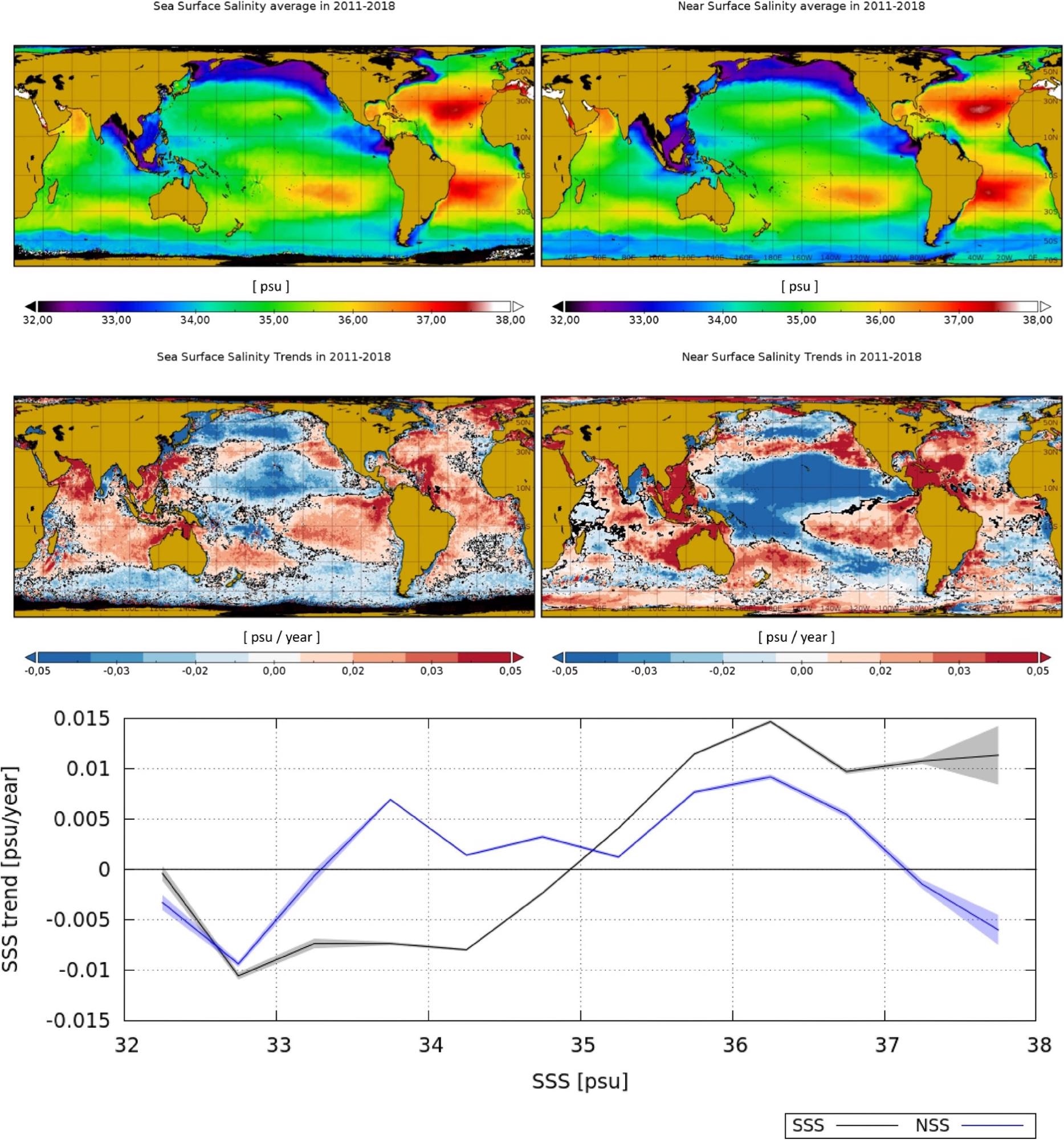
Figure 2. Top row: salinity average in 2011–2018 as observed by the satellite (SSS) (left) and by the model (NSS) (right). Middle row: satellite SSS trends (left) and model NSS trends (right) in 2011–2018. Locations with trends being different from zero with a 95% level of confidence are represented in black. Bottom plot: mean SSS (black) and NSS (blue) trend as a function of averaged SSS and NSS (respectively) in the same period. The shadowed area represents the confidence interval of the 95%. Maps are plotted with Panoply v 4.12.0. Image Credit: Olmedo, et al., 2022

Differences in SSS and NSS trends (upper left panel in Figure 3) demonstrate a large ocean area in the Pacific Ocean (between 30° S and 10° S) where SSS has a substantially less freshening tendency than NSS.

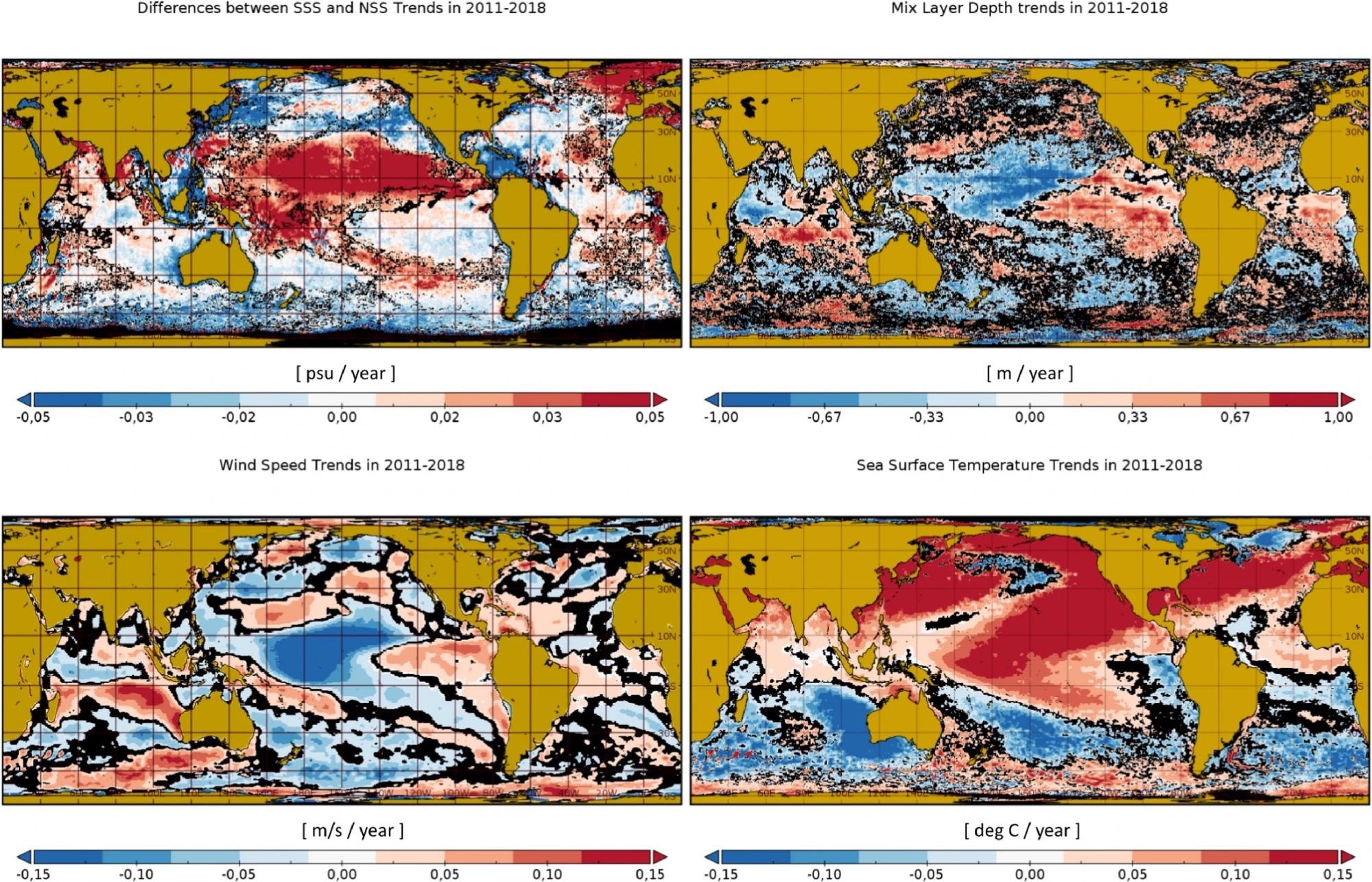
Figure 3. Top left panel: Differences between the satellite SSS trends and the model NSS trends in 2011–2018. Top right panel: mixed layer depth trends in 2011–2018. Bottom row: wind speed trends (left) and sea surface temperature trends in the same period (right). Locations with trends being different from zero with a 95% level of confidence are represented in black. Maps are plotted with Panoply v 4.12.0. Image Credit: Olmedo, et al., 2022

Negative discrepancies between SSS and NSS trends are offset by far more frequent positive ones, resulting in positive values when averaged across any region specified by a given value of MLD trend; hence, the SSS-NSS average trend panel on the top of Figure 4 only shows positive values.

​​​​​​​

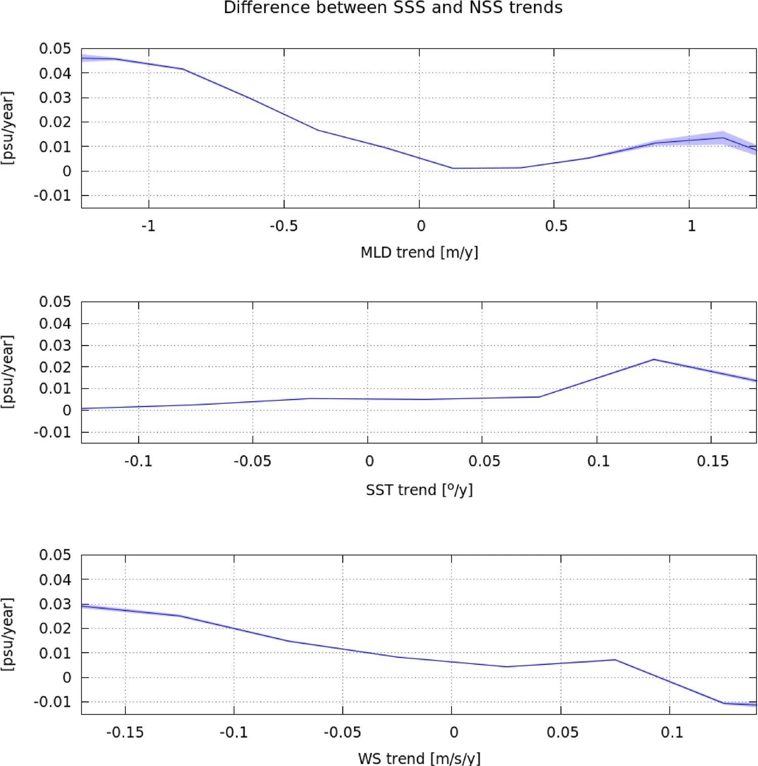
Figure 4. Mean difference between SSS and NSS trends as function of the following trends: mixed layer depth (top panel), sea surface temperature (middle panel), and wind speed (bottom panel). The region considered comprises tropics and middle latitudes (i.e., between 40° N and 40° ​​​​​​​S) to exclude from this analysis ocean regions that may be affected by sea-ice dynamics. Image Credit: Olmedo, et al., 2022

Discussion

Satellite data give a one-of-a-kind source of information on ocean mesoscale dynamics in the top layer that is unavailable from any other source (either models or in situ). They produce regular, global salinity maps that reach coastal and polar areas, greatly aiding in understanding sea surface salinity dynamics.

Aside from that, satellites measure SSS, distinct from the NSS observed in situ or predicted by models. As a result, satellite observations are complementary to in situ measurements.

According to the Clausius–Clapeyron (CC) connection, which indicates that the saturation of water vapor pressure rises at a rate of 7% each degree Celsius of warming, the water cycle is projected to intensify in a global warming scenario. In the face of climate change, this results in the “Dry Gets Drier and Wet Gets Wetter” (DDWW) paradigm.

Conclusion

These findings reveal that in locations with SSS of more than 34.7 psu, the positive trend dominates and the worldwide average is positive, but in places with SSS of less than 34.7 psu, the opposite is true, which is consistent with the DDWW paradigm. The NSS, on the other hand, does not demonstrate this amplification. This supports utilizing SSS (rather than NSS) as an E–P proxy.

Researchers see significant discrepancies between SSS and NSS trends in tropical and mid-latitude regions, most likely the result of a net stratification effect caused by surface warming. Under low wind circumstances, the consistent rise in temperature forms a warm layer in the top few meters of the ocean, where the temperature rises towards the surface.

Evaporation from the ocean surface is favored because these circumstances persist throughout time. As a result, SSS increases in comparison to NSS.

Journal Reference:

Olmedo, E., Turiel, A., González-Gambau, V., González-Haro, C., García-Espriu, A., Gabarró, C., Portabella, M., Corbella, I., Martín-Neira, M., Arias, M. and Catany, R. (2022) Increasing stratification as observed by satellite sea surface salinity measurements. Scientific reports, 12(1), pp.1-9. Available Online: https://www.nature.com/articles/s41598-022-10265-1.

References and Further Reading

1. Schmitt, R W (2008) Salinity and the global water cycle.Oceanography, 21(1), pp. 12–19. doi.org/10.5670/oceanog.2008.63.
2. Durack, P., et al. (2012) Ocean salinities reveal strong global water cycle intensification during 1950 to 2000.Science,336(6080), pp. 455–458. doi.org/10.1126/science.1212222.
3. Huntington, T (2006) Evidence for intensification of the global water cycle: Review and synthesis.Journal of Hydrology,319(1–4), pp. 83–95. doi.org/10.1016/j.jhydrol.2005.07.003.
4. Allen, M R & Ingram, W (2002) Constraints on future changes in climate and the hydrologic cycle.Nature,419, pp. 228–232. doi.org/10.1038/nature01092.
5. Held, I & Soden, B (2006) Robust responses of the hydrological cycle to global warming. Journal of Climate,19(21), pp. 5686–5699. doi.org/10.1175/JCLI3990.1.
6. Trenberth, K., et al. (2005) Trends and variability in column-integrated atmospheric water vapor. Climate Dynamics, 24, pp. 741–758. doi.org/10.1007/s00382-005-0017-4.
7. Allan, R & Soden, B (2008) Atmospheric warming and the amplification of precipitation extremes. Science, 321, pp. 481–1484.
8. Yu, L. (2007) Global variations in oceanic evaporation (1958–2005): The role of the changing wind speed. The Journal of Climate, 20, pp. 5376–5390. doi.org/10.1175/2007JCLI1714.1.
9. Zhang, Y., et al. (2016) Multi-decadal trends in global terrestrial evapotranspiration and its components. Scientific Reports, 6, p. 19124. doi.org/10.1038/srep19124.
10. Yu, L., et al. (2020) Intensification of the global water cycle and evidence from ocean salinity: Synthesis review. Annals of the New York Academy of Sciences, 1472, pp. 76–94. doi.org/10.1111/nyas.14354.
11. Helm, K. P., et al. (2010) Changes in the global hydrological-cycle inferred from ocean salinity. Geophysical Research Letters, 37, p. L18701. https://doi.org/10.1029/2010GL044222.
12. Skliris, N., et al. (2016) Global water cycle amplifying at half Clausius–Clapeyron rate. Scientific Reports, p. 38752. doi.org/10.1038/srep38752.
13. Vinogradova, N & Ponte, P (2017) In search of finger-prints of the recent intensification of the ocean water cycle. The Journal of Climate, 30, pp. 5513–5528. doi.org/10.1175/JCLI-D-16-0626.1.
14. Zika, J. D., et al. (2015) Maintenance and broadening of the ocean’s salinity distribution by the water cycle. The Journal of Climate, 28, pp. 9550–9560. doi.org/10.1175/JCLI-D-15-0273.1.
15. Zika, J. et al. (2018) Improved estimates of water cycle change from ocean salinity: The key role of ocean warming. Environmental Research Letters, 13, p. 74036.
16. Yu, L (2011) A global relationship between the ocean water cycle and near-surface salinity. Journal of Geophysical Research, 116, p. C10025. doi.org/10.1029/2010JC006937.
17. Mignot, J & Frankignoul, C (2003) On the interannual variability of surface salinity in the Atlantic. Climate Dynamics, 20, pp. 555–565. doi.org/10.1007/s00382-002-0294-0.
18. Mignot, J & Frankignoul, C (2004) Interannual to inter-decadal variability of sea surface salinity in the Atlantic and its link to the atmosphere in a coupled model. Journal of Geophysical Research, 109, p. C04005. doi.org/10.1029/2003JC002005.
19. Bingham, F. M., et al. (2002) Sea surface salinity measurements in the historical database. Journal of Geophysical Research, 107, pp. SRF 20-1-SRF 20-10. doi.org/10.1029/2000JC000767.
20. Argo. Argo, 2000. (2021) Argo Float Data and Metadata From Global Data Assembly Centre (Argo GDAC). SENOE. doi.org/10.17882/42182.
21. Mecklenburg, S., et al. (2012) ESA’s soil moisture and ocean salinity mission: Mission performance and operations. IEEE Transactions on Geoscience and Remote Sensing, 50, pp. 1354–1366. doi.org/10.1109/TGRS.2012.2187666.
22. Lagerloef, G., et al. (2008) The aquarius/SAC-D mission—Designed to meet the salinity remote sensing challenge. Oceanographic Magazine, 21, pp. 68–81.
23. Entekhabi, D. et al. (2010) The soil moisture active passive (SMAP) mission. Proceedings of the IEEE, 98, pp. 704–716. doi.org/10.1109/JPROC.2010.2043918.
24. Donlon, C. J., et al. (2002) Toward improved validation of satellite sea surface skin temperature measurements for climate research. The Journal of Climate, 15, pp. 353–369. doi.org/10.1175/1520-0442(2002)015%3C0353:TIVOSS%3E2.0.CO;2.
25. Ward, B (2006) Near-surface ocean temperature. Journal of Geophysical Research, 111, pp. 1–18. doi.org/10.1029/2004JC002689.
26. Maes, C & O’Kane, T. J (2014) Seasonal variations of the upper ocean salinity stratification in the tropics. Journal of Geophysical Research Oceans, 119, pp. 1706–1722. https://doi.org/10.1002/2013JC009366.
27. Boutin, J., et al. (2016) Satellite and in situ salinity: Understanding near-surface stratification and sub-footprint variability. Bulletin of the American Meteorological Society, 97, pp. 1391–1407. doi.org/10.1175/BAMS-D-15-00032.1.
28. Webster, P. J., et al. (2002) The JASMINE pilot study. Bulletin of the American Meteorological Society, 83, pp. 1603–1630. https://doi.org/10.1175/BAMS-83-11-1603.
29. Anderson, J E & Riser, S C (2014) Near-surface variability of temperature and salinity in the near-tropical ocean: Observations from profiling floats. Journal of Geophysical Research Oceans, 119, pp. 7433–7448. doi.org/10.1002/2014JC010112.
30. Ward, B., et al. (2014) The Air–Sea Interaction Profiler (ASIP): An autonomous upwardly rising profiler for microstructure measurements in the upper ocean. The Journal of Atmospheric and Oceanic Technology, 31, pp. 2246–2267. doi.org/10.1175/JTECH-D-14-00010.1.
31. Walesby, K., et al. (2015) Observations indicative of rain-induced double diffusion in the ocean surface boundary layer. Geophysical Research Letters, 42, pp. 3963–3972. doi.org/10.1002/2015GL063506.
32. Sutherland, G., et al. (2014) Mixed and mixing layer depths in the ocean surface boundary layer under conditions of diurnal stratification. Geophysical Research Letters, 41, pp. 8469–8476. doi.org/10.1002/2014GL061939.
33. Reverdin, G., et al. (2012) Rain-induced variability of near sea-surface t and s from drifter data. Journal of Geophysical Research Oceans, doi.org/10.1029/2011JC007549.
34. Drucker, R & Riser, S C (2014) Validation of aquarius sea surface salinity with ARGO: Analysis of error due to depth of measurement and vertical salinity stratification. Journal of Geophysical Research Oceans, 119, pp. 4626–4637. doi.org/10.1002/2014JC010045.
35. Henocq, C., et al. (2010) Vertical variability of near-surface salinity in the tropics: Consequences for L-band radiometer calibration and validation. The Journal of Atmospheric and Oceanic Technology, 27, pp. 192–209. doi.org/10.1175/2009JTECHO670.1.
36. Volkov, D. L., et al. (2019) Observations of near-surface salinity and temperature structure with dual-sensor Lagrangian drifters during SPURS-2. Oceanography, 32, pp. 66–75.
37. Sprintall, J & Tomczak, M (1992) Evidence of the barrier layer in the surface layer of the tropics. Journal of Geophysical Research Oceans, 97, pp. 7305–7316. doi.org/10.1029/92JC00407.
38. Pailler, K., et al. (1999) The barrier layer in the western tropical Atlantic Ocean. Geophysical Research Letters, 26, pp. 2069–2072. doi.org/10.1029/1999GL900492.
39. Mignot, J., et al. (2007) Control of salinity on the mixed layer depth in the world ocean: 2. Tropical areas. Journal of Geophysical Research Oceans, doi.org/10.1029/2006JC003954.
40. Straneo, F & Heimbach, P (2013) North Atlantic warming and the retreat of Greenland’s outlet glaciers. Nature, 504, pp. 36–43. doi.org/10.1038/nature12854.
41. Nicholls, K. W., et al. (2009) Ice-ocean processes over the continental shelf of the southern Weddell Sea, Antarctica: A review. Reviews of Geophysics, doi.org/10.1029/2007RG000250.
42. Marsh, R., et al. (2010) Short-term impacts of enhanced greenland freshwater fluxes in an eddy-permitting ocean model. Ocean Science, 6, pp. 749–760. doi.org/10.5194/os-6-749-2010.
43. Yu, L (2010) On sea surface salinity skin effect induced by evaporation and implications for remote sensing of ocean salinity. Journal of Physical Oceanography, 4, pp. 85–102. doi.org/10.1175/2009JPO4168.1.
44. Asher, W. E., et al. (2014) Stable near-surface ocean salinity stratifications due to evaporation observed during strasse. Journal of Geophysical Research Oceans, 119, pp. 3219–3233. doi.org/10.1002/2014JC009808.
45. Hodges, B A & Fratantoni, M D (2014) Auv observations of the diurnal surface layer in the north Atlantic salinity maximum. Journal of Physical Oceanography, 44, pp. 1595–1604. doi.org/10.1175/JPO-D-13-0140.1.
46. Stevens, C., et al. (2011) Surface layer mixing during the SAGE ocean fertilization experiment. Deep-Sea Research Part II: Topical Studies in Oceanography, 58, pp. 776–785. doi.org/10.1016/j.dsr2.2010.10.017.
47. Sutherland, G., et al. (2014) Evaluating Langmuir turbulence parameterizations in the ocean surface boundary layer. Journal of Geophysical Research: Oceans, 119, pp. 1899–1910. doi.org/10.1002/2013JC009537.
48. Olmedo, E., et al. (2021) Nine years of SMOS sea surface salinity global maps at the Barcelona Expert Center. Earth System Science Data, 13, pp. 857–888. doi.org/10.5194/essd-13-857-2021.
49. Olmedo, E., et al. (2017) Debiased non-Bayesian retrieval: A novel approach to SMOS Sea Surface Salinity. Remote Sens. Environ. 193, 103–126. doi.org/10.1016/j.rse.2017.02.023.
50. Zweng, M. M. et al. (2013) World Ocean Atlas 2013, Volume 2: Salinity 74 (eds. Levitus, A., Mishonov Technical Ed.) (NOAA Atlas NESDIS).