Local and national government bodies are increasingly stipulating that processing companies monitor the different emissions from their plant stacks and flares in order to decrease pollution entering the atmosphere.
Focus was initially on oil refinery flares, but this has recently shifted to petrochemical and chemical plant flares as potential sources of hazardous air pollutants.
Petrochemical Plants
The Environmental Protection Agency (EPA) signed off a range of Risk and Technology Review (RTR) rules in March 2020, including the National Emission Standards for Hazardous Air Pollutants (NESHAP) and the Generic Maximum Achievable Control Technology Standards for Ethylene Production (EMACT).
The requirements in place for EMACT flares were deemed to be inadequate in meeting the need to ensure 98 % destruction efficiency required by the standards. EMACT flares must now be monitored continuously, as these are subject to the same flare requirements and definitions as refineries.
Existing ethylene crackers are required to be compliant within three years following the publication of the final rule in the Federal Register. New crackers or facilities that began construction after October 9, 2019, are required to comply on initial start-up or on the date of publication of the final rule, whichever is later.
Organic Chemicals Manufacturers
Amendments to the 2003 Miscellaneous Organic Chemical Manufacturing National Emission Standards for Hazardous Air Pollutants (NESHAP), known as MON, were finalized by EPA in May 2020.
These amendments add new monitoring and operational requirements for flares controlling emissions from processes generating olefins and polyolefins, as well as flares controlling ethylene oxide emissions.
The amendments also allow facilities outside of this subset to opt into these flare control requirements instead of maintaining compliance with current flare standards.
These finalized amendments are expected to decrease hazardous air pollutant (HAP) emissions by 107 tons per year, with reductions in ethylene oxide emissions estimated to be around 0.76 tons per year. HAP emissions from flares are also expected to decrease by around a further 260 tons per year.
Oil Refineries
These new rules follow rules published in November 2018, when amendments were introduced to the Refinery Sector Rule (RSR) 40 CFR Part 63, which required refineries to bring flares into compliance with new §63.670, ‘Requirements for Flare Control Devices,’ by January 30, 2019.
These new requirements define a total of five flare operating limits:
- Dilution net heating value (NHVdil)
- Combustion zone net heating value (NHVCZ)
- Visible emissions
- Flare tip exit velocity
- Pilot flame presence
An NHVCZ minimum operating limit of 270 BTU/scf is also specified based on a 15-minute block period.1
Flare gas analysis should be a key part of any compliance strategy. For example, NHVCZ can be calculated by measuring the net heating value of the vent gas (NHVVG), adding further fuel gas such as natural gas or propane if the NHVCZ approaches 270 BTU/scf. Steam may also need to be added to the flare to avoid the production of visible emissions.
Measurement of Flare Gas Streams by Process Mass Spectrometry
Flare gas analysis is accompanied by a range of challenges, irrespective of what process the gases originate from. Emissions are typically comprised of complex mixtures of organic and inorganic species, with concentrations and compositions of these species altering significantly over time as process conditions change.
Many regulations only require the capture of total heating value, total sulfur, or total hydrocarbon values, but measuring individual component concentrations helps to identify the source of the emission, locating the specific part of the plant that is causing a problem.
Analysis speed is also vital, because the flare’s heating value can change quickly, with analysis times measured in minutes likely to fall short of emission standards.
Process Mass Spectrometry is especially suited to the measurement of flare gas streams, due to its capacity to provide rapid, accurate, multicomponent analysis. Table 1 features an example of a flare gas stream that contains nitrogen, hydrogen, and hydrocarbons up to C6.
It typically takes less than 30 seconds to analyze these 19 components, meaning that a single mass spectrometer can be used to monitor multiple flares, depending on the distances involved.
Advantages of the Prima PRO Process Mass Spectrometer
A magnetic sector analyzer forms the core of the Thermo Fisher Scientific™ Prima PRO Process Mass Spectrometer (Figure 1), offering unparalleled precision and accuracy versus other mass spectrometers.
Table 1. Example of flare gas stream composition. Source: Thermo Fisher Scientific – Environmental and Process Monitoring Instruments
| Component |
Molecular Weight |
Flare Gas Typical Composition %mol |
| Hydrogen |
2 |
0-40 |
| Methane |
16 |
15-95 |
| Water |
18 |
0-8 |
Carbon
Monoxide |
28 |
0-1 |
| Nitrogen |
28 |
0-40 |
| Ethylene |
28 |
0-12 |
| Ethane |
30 |
2-15 |
| Oxygen |
32 |
0-5 |
Hydrogen
Sulfide |
34 |
0-10 |
| Propylene |
42 |
0-20 |
Carbon
Dioxide |
44 |
0-10 |
| Propane |
44 |
0-5 |
| 1-3, Butadiene |
54 |
0-0.2 |
| Butenes |
56 |
0-15 |
| i-Butane |
58 |
0-10 |
| n-Butane |
58 |
0-5 |
| C5 and C6 |
70+ |
0-15 |
Carbonyl
Sulfide |
60 |
0-10 ppm |
Carbon
Disulfide |
76 |
0-1 ppm |
The company manufactures both quadrupole and magnetic sector mass spectrometers, boasting over 30 years of industrial experience, demonstrating that the magnetic sector-based analyzer offers the best performance for industrial online gas analysis.
There are several benefits to using magnetic sector analyzers, including:
- Long intervals between calibrations
- Resistance to contamination
- Improved precision
- Excellent accuracy
The analytical precision of these instruments is typically between two and 10 times better than that of a quadrupole analyzer, depending on the complexity of the mixture and the gases analyzed.
The system works by initially converting neutral gas atoms and molecules into positively charged ions in the Prima PRO Process Mass Spectrometer ion source. This enclosed source ensures high sensitivity, minimum background interference, and maximum contamination resistance.
The Prima PRO Process Mass Spectrometer’s high-energy (1000 eV) analyzer delivers extremely robust performance in the presence of gases and vapors with the potential to contaminate internal vacuum components.
It has a proven track record of monitoring high percent level concentrations of organic compounds without experiencing drift or contamination.
Ions are then accelerated through a flight tube, separated by their mass-to-charge ratios in a magnetic field of variable strength. Because the magnetic sector mass spectrometer produces a focused ion beam at the detector, the peak shape produced via this process is ‘flat-topped’, and uniform response is seen over a finite mass width.
The peak’s height is directly proportional to the number of ions striking the detector, meaning that it is also directly proportional to the concentration of the component being measured.
The high precision analysis is ensured so long as the measurement is acquired anywhere on the peak’s flat top.
The Prima PRO Process Mass Spectrometer’s ability to measure over a wide dynamic range is key to accurately measuring the varying composition levels in flare gas.
The instrument was independently evaluated by EffecTech UK, an independent specialist company that provides accredited calibration and testing services to the power and energy industries for gas flow, quality, and total energy metering.
The company is accredited to internationally recognized ISO/IEC 17025:2005 standards. These standards specify the general competence requirements to perform tests and/or calibrations, including sampling.
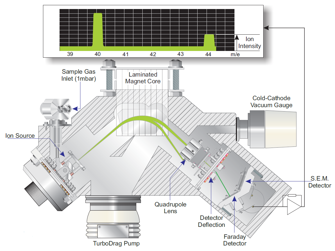
Figure 1. Prima PRO Process Mass Spectrometer magnetic sector analyzer. Image Credit: Thermo Fisher Scientific – Environmental and Process Monitoring Instruments
Rapid Multistream Sampling
Multistream sampling is a quick, reliable means of switching between streams in scenarios where the mass spectrometer is required to monitor multiple flare streams or a combination of flare streams and process streams.
Solenoid valve manifolds have too much dead volume, and rotary valves suffer from poor reliability. These limitations prompted Thermo Fisher Scientific to develop its unique Rapid Multistream Sampler (RMS).
The RMS provides an unrivaled combination of sampling speed and reliability, enabling sample selection from one of 32 or one of 64 streams. The user has full control over stream settling times, meaning these are fully configurable and application dependent. Digital sample flow recording is also performed for each stream selected.
An alarm can be triggered if the sample flow drops, for instance, if a filter in the sample conditioning system becomes blocked. The stream selector’s position is optically encoded, and the RMS can be heated to 120 °C to ensure reliable, software-controlled stream selection.
Temperature and position control signals are communicated via the Prima PRO Process Mass Spectrometer’s internal network.
The RMS has a proven track record of performing 10 million operations between maintenance and comes complete with a three-year warranty as standard. No other multi-stream sampling device has the same level of guaranteed reliability.
Measuring Fuel Properties with Prima Pro Process Mass Spectrometer
The Prima PRO Process Mass Spectrometer can be used to routinely measure an array of fuel properties.
Source: Thermo Fisher Scientific – Environmental and Process Monitoring Instruments
| . |
. |
| Lower Heating Value (LHV) |
Also known as Net Heating Value or
Lower Calorific Value |
| Higher Heating Value (HHV) |
Also known as Gross Heating Value or
Higher Calorific Value |
| Compressibility |
|
| Actual Lower Heating Value |
Ideal Lower Heating Value
--------------------------------------
Compressibility |
| Density |
|
| Specific Gravity |
|
| Lower Wobbe Index |
Lower Heating Value
--------------------------------
√(Specific Gravity) |
| Higher Wobbe Index |
Higher Heating Value
----------------------------------
√(Specific Gravity) |
| Air Requirement |
|
| Combustion Air Requirement Index (CARI) |
Air Requirement
-----------------------------
√(Specific Gravity) |
Lower Heating Value (LHV) is calculated using the value of 1212 BTU/scf for hydrogen instead of the theoretical value of 274 BTU/scf. This approach is recommended by EPA 40 CFR Parts 60 and 63, and supplies the user with a more reliable indication of flare performance (for instance, whether the flare meets the minimum operating limit of 270 BTU/scf).
The accurate analysis of hydrogen across a wide dynamic range is vital due to its high combustion potential. The Prima PRO Process Mass Spectrometer’s magnetic sector analyzer is ideally suited to hydrogen analysis because it does not suffer from the ‘zero blast,’ a phenomenon that hinders the analysis of light molecules on many quadrupole analyzers.
HHV is different from LHV in that it considers the latent heat of vaporization of water in the combustion process. When using the Prima PRO model, the precision of these measurements is usually better than 0.1 % relative.
Figure 2 outlines how the ideal LHV of the flare gas stream is calculated by the GasWorks software. Derived values are based on the individual components’ ideal LHVs.
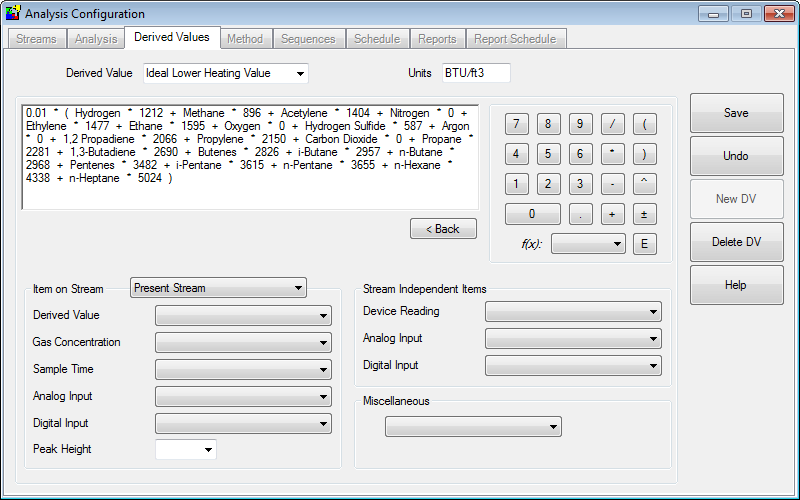
Figure 2. GasWorks Derived Value for Ideal Lower Heating Value. Image Credit: Thermo Fisher Scientific – Environmental and Process Monitoring Instruments
Analysis times are typically 30 seconds or less, including settling time. Data is communicated to the plant host computer because this can be measured by various techniques, including 4–20 mA or 0–10 V analog outputs, Modbus, Profibus, or OPC.
Analytical Setup
The GasWorks software supports an unlimited number of analysis techniques, allowing the analysis to be optimized on a per-stream basis. The most appropriate speed versus precision settings and the most efficient peak measurements can be chosen for each gas stream, depending on process control requirements.
Figures 3 and 4 feature examples of different analysis techniques: Figure 3 shows an example of the analytical technique for a flare gas stream, while Figure 4 demonstrates the technique for a process stream.
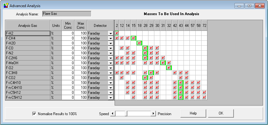
Figure 3. Example of flare stream method. Image Credit: Thermo Fisher Scientific – Environmental and Process Monitoring Instruments
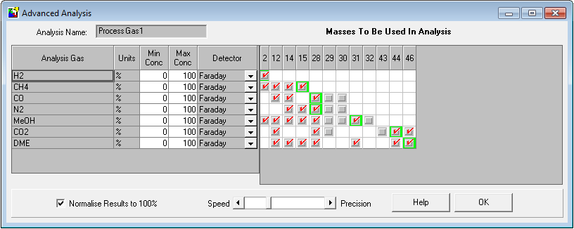
Figure 4. Example of process stream method. Image Credit: Thermo Fisher Scientific – Environmental and Process Monitoring Instruments
Both of these approaches (and additional process techniques) are being performed by using a single Prima PRO Process Mass Spectrometer to measure a combination of flare gas and process streams.
These two techniques also clearly demonstrate the degree of spectral overlap in the MS fragmentation patterns. It is important to measure these fragmentation patterns separately from the components of interest. The use of surrogate compounds may simplify the calibration process, but this will inevitably lead to decreased accuracy.
Flare Gas Test Data
A factory test was performed on the Prima PRO Process Mass Spectrometer to check the performance on a refinery flare gas application. This was done on a gravimetric cylinder containing 21 components, including inorganics and hydrocarbons from C1 to C6.
Table 2. Factory test on a gravimetric cylinder containing 21 inorganic and hydrocarbon compounds, analyzed over 18 hours. Source: Thermo Fisher Scientific – Environmental and Process Monitoring Instruments
| Component |
Concentration
%mol |
Prima PRO Specification
for Standard Deviation
%mol (8 hours) |
FAT test Ave
%mol (8 hours) |
FAT Test
Actual Standard Deviation
%mol (8 hours) |
| Hydrogen |
10 |
≤ 0.02 |
9.8835 |
0.0077 |
| Methane |
64.53 |
≤ 0.05 |
64.6662 |
0.0125 |
Carbon
Monoxide |
5 |
≤ 0.05 |
5.0829 |
0.0264 |
| Nitrogen |
10 |
≤ 0.05 |
9.8557 |
0.0469 |
| Ethylene |
2 |
≤ 0.02 |
1.9867 |
0.0010 |
| Ethane |
2 |
≤ 0.02 |
2.0367 |
0.0012 |
| Oxygen |
1 |
≤ 0.001 |
0.9941 |
0.0006 |
Hydrogen
Sulfide |
0.05 |
≤ 0.0005 |
0.0484 |
0.0003 |
| Propylene |
1 |
≤ 0.001 |
0.9961 |
0.0011 |
Carbon
Dioxide |
1 |
≤ 0.001 |
0.9597 |
0.0007 |
| Propane |
1 |
≤ 0.001 |
1.0910 |
0.0007 |
| 1,3 Butadiene |
0.1 |
≤ 0.005 |
0.0992 |
0.0003 |
| Butenes |
0.5 |
≤ 0.005 |
0.5023 |
0.0005 |
| i-Butane |
0.5 |
≤ 0.005 |
0.4892 |
0.0011 |
| n-Butane |
0.5 |
≤ 0.005 |
0.5059 |
0.0026 |
Carbonyl
Sulfide |
100 ppm |
≤ 1 ppm |
100.5319 |
0.4470 |
| Pentenes |
0.1 |
≤ 0.005 |
0.0992 |
0.0004 |
| i-Pentane |
0.3 |
≤ 0.005 |
0.3083 |
0.0012 |
| n-Pentane |
0.3 |
≤ 0.005 |
0.2792 |
0.0042 |
Carbon
Disulfide |
100 ppm |
≤ 1 ppm |
100.4589 |
0.2733 |
| n-Hexane |
0.1 |
≤ 0.005 |
0.0957 |
0.0010 |
| NHV (BTU/scf) |
|
≤ 0.1 % relative |
899.5394 |
0.07 % |
Table 3 shows the Prima PRO Process Mass Spectrometer’s quoted performance (including standard deviation over eight hours), the composition of the cylinder, and the results from the test itself.
The measured standard deviations for all 21 components were found to be less than the specified standard deviations over the eight-hour period.
The Prima PRO Process Mass Spectrometer also calculated the Net Heating Value over the eight hours of the test. Like the component concentrations, the measured NHV standard deviations were determined to be far less than the specified eight-hour standard deviations.
Figures 5a to 5d show trend data for minor components, major components, sulfur components, and NHV over the eight hours of the test.
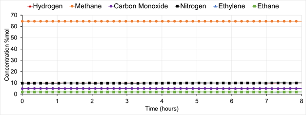
Figure 5a. Major component concentrations obtained during factory test on a gravimetric cylinder containing 21 inorganic and hydrocarbon compounds, analyzed over 8 hours. Image Credit: Thermo Fisher Scientific – Environmental and Process Monitoring Instruments
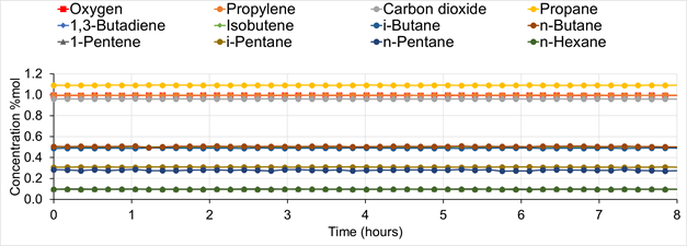
Figure 5b. Major component concentrations obtained during factory test on a gravimetric cylinder containing 21 inorganic & hydrocarbon compounds, analyzed over 8 hours. Image Credit: Thermo Fisher Scientific – Environmental and Process Monitoring Instruments
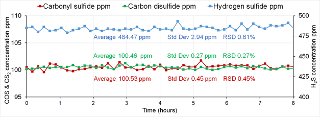
Figure 5c. Sulfur component concentrations obtained during factory test on a gravimetric cylinder containing 21 inorganic & hydrocarbon compounds, analyzed over 8 hours. Image Credit: Thermo Fisher Scientific – Environmental and Process Monitoring Instruments
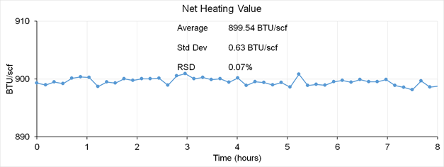
Figure 5d. NHV obtained during factory test on a gravimetric cylinder containing 21 inorganic & hydrocarbon compounds, analyzed over 8 hours. Image Credit: Thermo Fisher Scientific – Environmental and Process Monitoring Instruments
Analysis of Total Sulfur
Refinery regulators tend to be primarily interested in Total Reduced Sulfur (TRS) and hydrogen sulfide (H2S) values, but there is a degree of divergence on what constitutes TRS.
TRS is defined as H2S together with carbonyl sulfide (COS) and carbon disulfide (CS2) in some cases. Alternatively, it can be defined as a mixture of compounds that contain a sulfur component in its reduced form, generally, H2S, methanethiol (methyl mercaptan, CH3SH), dimethyl sulfide (DMS, (CH3)2S), and dimethyl disulfide (DMDS, CH3S2CH3).
Mass spectrometers can quantify a range of sulfur compounds down to ppm levels. Table 4 features typical performance figures for the Prima PRO Process Mass Spectrometer. Analysis time is less than 30 seconds, including stream switching time and standard deviations measured over a period of eight hours.
Table 3. Typical Prima PRO Process Mass Spectrometer performance specification for sulfur compounds. Source: Thermo Fisher Scientific – Environmental and Process Monitoring Instruments
| Component |
Typical Composition
%mol |
Precision of analysis by
Prima PRO Process MS
(single standard deviation) ≤ |
| Hydrogen Sulfide |
3 ppm |
0.5 ppm |
| Methyl Mercaptan |
10 ppm |
0.5 ppm |
| Ethyl Mercaptan |
10 ppm |
0.5 ppm |
| n-Propyl Mercaptan |
10 ppm |
0.5 ppm |
| n-Butyl Mercaptan |
10 ppm |
0.5 ppm |
A unit was calibrated for hydrogen sulfide, carbonyl sulfide, and carbon disulfide at a single concentration. This was performed using three cylinders to highlight the excellent linearity of the Prima PRO Process Mass Spectrometer when analyzing sulfur species.
It was then used to analyze a series of cylinders containing the three sulfur species.
- COS was calibrated at 0.2006 %, with MS used to analyze COS concentrations from 0 % to 0.2006 %
- H2S was calibrated at 0.0506 %, with MS used to analyze H2S concentrations from 0 % to 89.88 %
- CS2 was calibrated at 0.198 %, with MS used to analyze CS2 concentrations from 0 % to 0.198 %
Table 4 shows the test gases used to demonstrate system linearity, with the calibration gases highlighted in red. The linearity achieved for the three sulfur species is demonstrated in Figure 6.
This data highlights the Prima PRO Process Mass Spectrometer’s capacity to measure up to 100 % concentrations and its ability to be safely calibrated for hydrogen sulfide at trace levels (0.05 % in this case).
Table 4. Sulfur test gases are used to demonstrate Prima PRO Process Mass Spectrometer linearity. Source: Thermo Fisher Scientific – Environmental and Process Monitoring Instruments
H2S Actual
Concentration %mol |
H2S Measured
Concentration %mol |
COS Actual Concentration %mol |
COS Measured Concentration %mol |
CS2 Actual Concentration %mol |
CS2 Measured Concentration %mol |
| 0 |
0.0001 |
0 |
0 |
0 |
0.0002 |
| 0.003 |
0.0028 |
0.003 |
0.0029 |
0.003 |
0.0039 |
| 0.0506 |
0.0503 |
0.0502 |
0.0513 |
0.0498 |
0.0576 |
| 0.2505 |
0.261 |
0.2006 |
0.2015 |
0.198 |
0.2006 |
| 0.4997 |
0.526 |
|
|
|
|
| 2 |
2.08 |
|
|
|
|
| 50.03 |
51.1 |
|
|
|
|
| 89.88 |
89.88 |
|
|
|
|
The GasWorks software can be used to produce a figure for total sulfur by employing its Derived Value option to sum individual component concentrations.
It is important to note that the value for total sulfur only represents the sum of the sulfur compounds analyzed via MS. Any unknown or unidentified compounds will not be reported.
Thermo Scientific recommends utilizing the Thermo Scientific SOLA iQ Flare System in order to ensure a true total sulfur reading. This system offers a robust solution for the accurate and continuous determination of total sulfur in flare gas streams.2
SOLA iQ Flare employs PUVF (pulsed ultraviolet fluorescence) spectrometry to calculate total sulfur.
All organically bound sulfur is initially converted to sulfur dioxide (SO2) via sample combustion. The irradiation of SO2 with ultraviolet light at a specific wavelength results in the formation of an excited form of SO2.
The emission of fluorescence or light then relaxes the excited SO2 to its ground state. The intensity of emitted light is directly proportional to the SO2 concentration, meaning that this represents the total sulfur concentration of the flare stack.
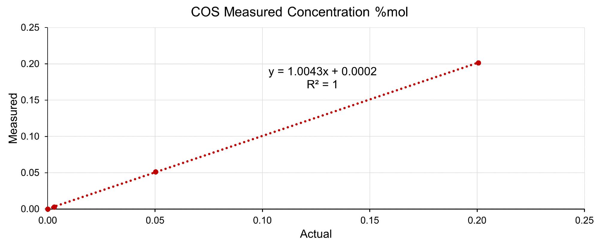
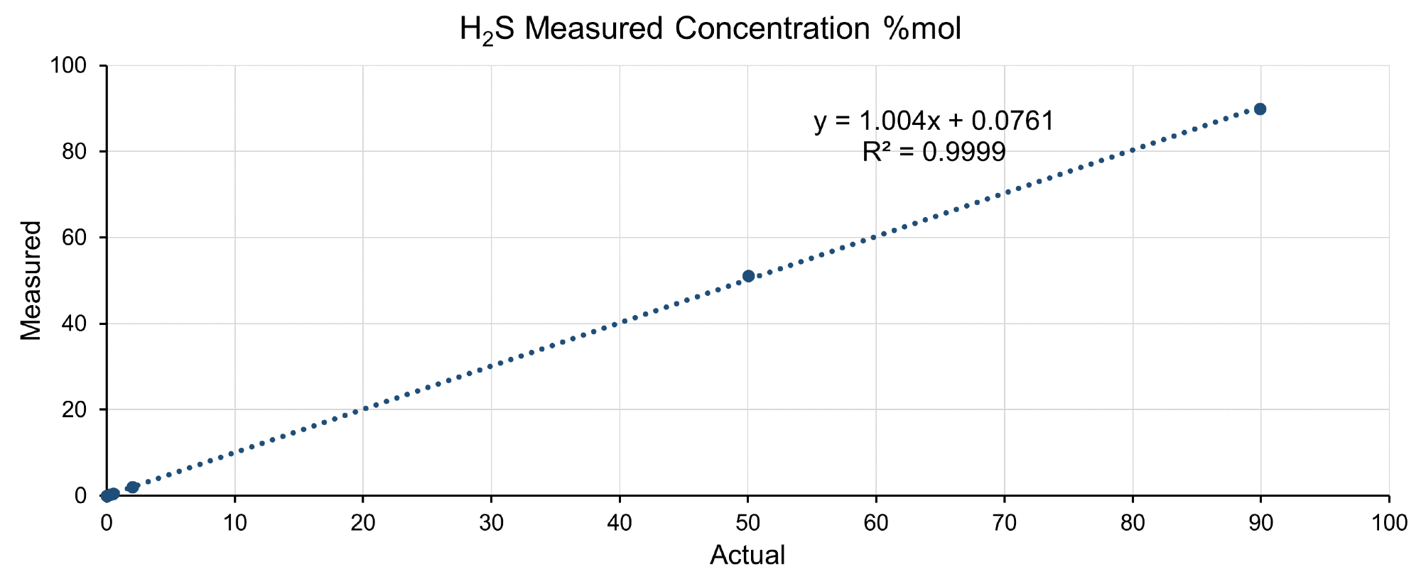
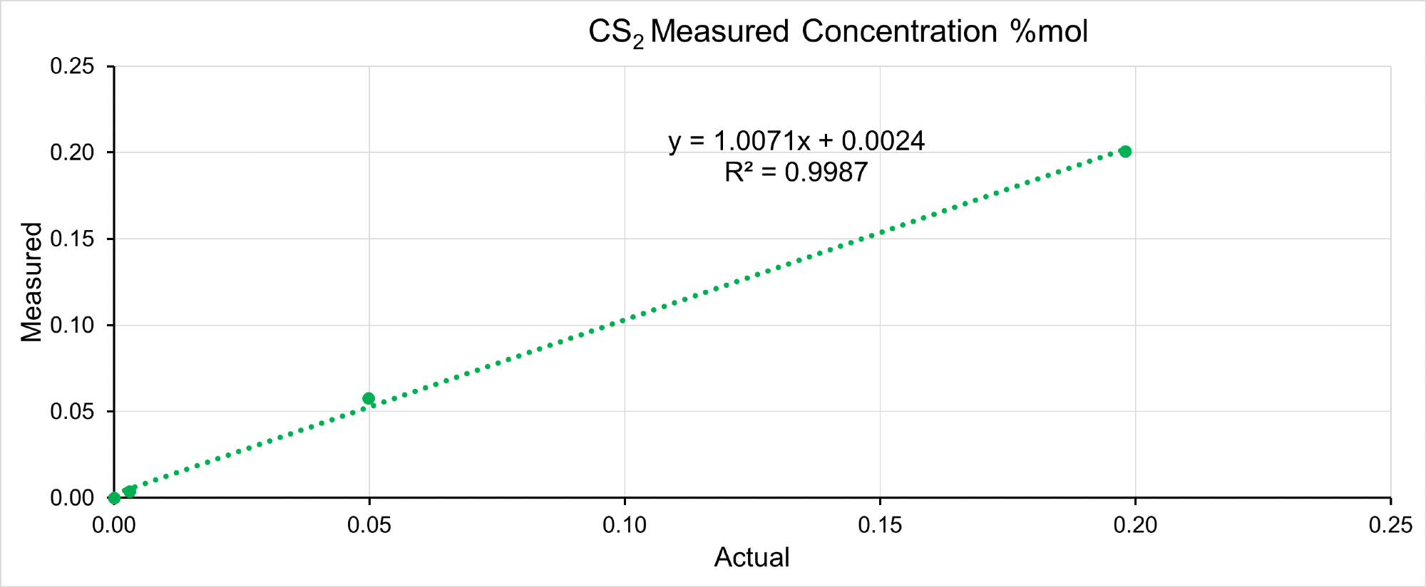
Figure 6. Prima PRO Process Mass Spectrometer linearity for hydrogen sulfide, carbonyl sulfide, and carbon disulfide. Image Credit: Thermo Fisher Scientific – Environmental and Process Monitoring Instruments
Summary
The Prima PRO Process Mass Spectrometer has had major success in the monitoring of refinery flare gases in recent years, delivering rapid, accurate online analysis of process gas composition and flare gas.
It also has a long and proven track record in the monitoring of ethylene furnaces and ethylene oxide processes,3,4 and is ideally suited to monitoring flare gas streams from these processes as concerns over hazardous emissions continue to increase.
When employed alongside the flexible GasWorks software, the inherent power of mass spectrometry allows a single Prima PRO Process Mass Spectrometer to monitor flare gas streams and multiple process streams. Comparing detailed composition data from the flare gas stream with that of multiple process streams is key to performing root cause fault analysis.
As well as complete compositional analysis, the Prima PRO Process Mass Spectrometer provides its users with accurate fuel gas properties, including HHV, LHV, density, specific gravity, stoichiometric air requirement, Wobbe Index, and CARI.
This robust measurement capability ensures that unburned pollutants are burnt to complete combustion rather than being emitted from flare waste gases.
References and Further Reading
- Govinfo. 40 CFR 63.670 -- Requirements for flare control devices. Available at: https://www.govinfo.gov/app/details/CFR-2025-title40-vol12/CFR-2025-title40-vol12-sec63-670.
- Merriman, D. Continuous flare stack emission monitoring: Thermo Scientific SOLA iQ Flare Analyzer. Thermo Fisher Scientific. Available at: https://documents.thermofisher.com/TFS-Assets/CAD/Application-Notes/sola-iq-flare%20stack%20monitoring-app-note.pdf.
- Thermo Fisher Scientific (2013). Advancing Process Control and Efficiency During Ethylene Production Using the Thermo Scientific Prima PRO Process Mass Spectrometer. Available at: https://gcms.labrulez.com/paper/33020.
- Thermo Fisher Scientific (2017). Thermo Scientific™ Prima PRO Process Mass Spectrometer - Improving ethylene oxide process control. Available at: https://gcms.cz/paper/33021.
Acknowledgments
Produced from materials originally authored by Dan Merriman from Thermo Scientific.

This information has been sourced, reviewed, and adapted from materials provided by Thermo Fisher Scientific – Environmental and Process Monitoring Instruments.
For more information on this source, please visit Thermo Fisher Scientific – Environmental and Process Monitoring Instruments.